
When numerically investigating vehicle aerodynamics with computational fluid dynamics (CFD), it can be useful to refer back to one of the reference vehicle geometries available in literature. This allows the setup of simulations to be tested on geometry for which both experimental and simulation data are available to compare against. Confident that the CFD is able to reproduce the data for such a reference body, one can then proceed to use CFD to extrapolate information about a vehicle geometry for which little to no data is available.
Several reference geometries exist, for example the Ahmed Body [1], the Society of Automotive Engineers (SAE) or Motor Industry Research Association (MIRA) reference bodies (with several geometry variations such as Notch-Back, Van, Fast-Back, Pick-Up) an overview of which can be found in [2] Le Good , or the modern DrivAer model [3].
This tutorial describes the setup of a simulation using the Ahmed Body at one Reynolds number. It can serve as a starting point for e.g. a mesh refinement study, turbulence model comparison or for a comparison of the effect of boundary condition.
Dimensions of the geometry used in the study
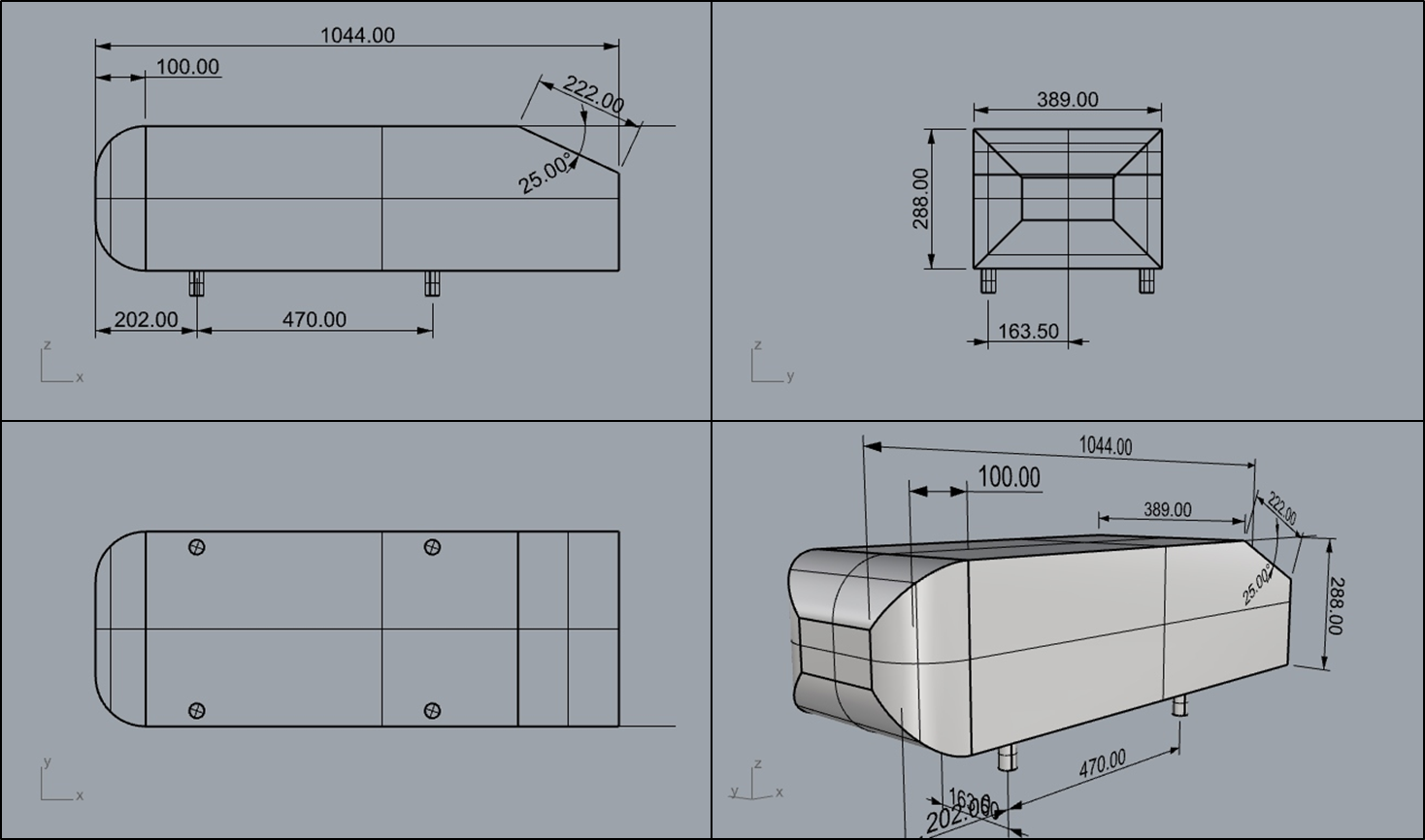
For this tutorial we are looking at an Ahmed Body with a rear end slant angle of 25 degrees.
Double click the .3dm file or drag and drop it into Rhino.
With GridSnap toggled on in Rhino, use the Move command to align the domain with the vehicle.
In the stl model provided, the vehicle should be aligned with World coordinates in Rhino thus making this task easier.
Position the vehicle approximately three vehicle lengths away from the inlet.
To check if GridSnap is on, simply type in GridSnap in the command bar.
The Box Edit tool may also be useful in aligning objects and domain exactly.
An inlet velocity of 10 m/s is set for the X-min domain face. The turbulence intensity should be set to something low or off (User-set defaults) to mimic the effect of the vehicle driving into quiescent air.
An open boundary is set for the X-max domain face.
The ground plane also has a velocity of 10m/s to simulate the car moving relative to the ground.
We change the box's type from being a Blockage to being a Null object - a Null object generates grid regions that are useful for setting up a refined mesh, but otherwise does not affect the simulation.
We also set the null objects view properties to wireframe for easier visualization
Meshing is not an exact science, it needs some experimentation to get good results. With that being said, we aim to have fine detail in the areas near the vehicle and less detail further away.
For this case, the mesh shown in the video was found to produce acceptable results. We recommend pausing the video when necessary.
Meshing can become a balance act between grid refinement and simulation time, and therefore sometimes the user may have to decide which one to prioritise.
We change the default settings for the solver to be more appropriate for aerodynamic problems.
If you are interested in learning more about the solvers and what happens under the hood we invite you to check out for solvers and POLIS as a gateway to everything else.
We change the default relaxation parameters to help the solver run faster for this specific case.
If you are interested in learning about convergence and relaxation we invite you to look at the Convergence page on POLIS .
When doing vehicle analysis such as this, it is best for the object of interest to be a single CAD object.
We then set up the reference parameters to calculate the drag coefficient.
Reference density is that of air, reference velocity is the same as the inlet, and the areas are the projected areas in each coordinate direction.
For more information about calculating drag coefficients have a look at the Forces on Objects POLIS page.
With the setup complete, we press run and let the computer do the heavy lifting!
This case has approximately 3.5 million cells, some complex vehicles may require even finer grids.
For reference, on a 16 core workstation with 4-channel memory (Threadripper 2950X) it took approximately 5 hours to complete. But on a more standard 4 core 2-memory channel office PC it could take much longer.
It is important to ensure that the solution has converged!
When the solution is converging we will observe a steadily decreasing residual plot during the runtime as shown in the adjacent image.
This case however has stagnated and will not converge further without making the mesh finer. For the purposes of the tutorial this is fine.
In most circumstances an unconverged solution is inaccurate and should not be used for decision making. For more information on convergence please look in our wiki entry.
Sometimes the flow dynamics are such that no steady-state can be achieved, then it may be necessary to run a transient simulation time-averaging the results to get the mean drag coefficient.
At the time of publication there is a known bug in RhinoCFD:
RhinoCFD adds both pressure and friction forces to the automated calculation of Cd. The values of pressure and friction force are listed separately inside the "result" file, so as a temporary measure we provide a .xlsl file to compute the correct Cd.
Under normal circumstances .csv files are produced that contain the Cd values.
The result file contains a lot of detailed information, for more information on this please see here.
In this simulation we obtained a Cdx of 0.396, which is close to the expected experimental result of 0.342 [4]. Further refining the grid improves the computed Cd value, indicating that the grid settings used for this tutorial are not yet fine enough for a detail study. With a grid of 231 x 182 x 119 and smaller cells (~20% smaller) near and on the walls of the Ahmed body, the computed Cdx value is 0.333, which compares well with the expected value.
Once the simulation is complete we can load up the results and check if everything in order.
Extract information from the model as needed. Have a look at this video for info on what post processing can be done in RhinoCFD.