       *************************************************************
       *                                                           *
       *   An application of the multi-fluid model of turbulence   *
       *   to the simulation of concentration fuctuations in       *
       *   isothermal confined jets.                               *
       *                                                           *
       *   by Sergei Zhubrin, Concentration, Heat and Momentum Ltd *
       *                                                           *
       *   June, 1997                                              *
       *************************************************************
A TURBULENCE MODEL FOR CONCENTRATION FLUCTUATIONS WHICH USES NO CONSERVATION EQUATIONS FOR STATISTICAL PROPERTIES OF THE FLUCTUATIONS is an application of Multi-Fluid concept of Spalding.
THE 1-, 3-, 5-, 9- and 17-FLUID MODELS are employed to simulate the TURBULENT MIXING RESULTING FROM THE ADMISSION OF TWO SEPARATE, ISOTHERMAL, COAXIAL JETS OF DIFFERENT COMPOSITION INTO A CONCENTRIC DUCT.
Appendix. Q1 file for 17 fluid model
       -----------------------------------------------------------------


     Entrance ///////////////////// Duct wall //////////////////Exit
              --->                         ::::::::::::          ->
  surrounding --->               ::::::::::                      -->
      jet     --------->:::::::::  Mixing layer spreading to wall--->
       "      --------->                                         ---->
  central jet --------->-.-.-.-.-.-.- Symmetry axis .-.-.-.-.-.-.----->


       -----------------------------------------------------------------
Each of the fluids has a DIFFERENT MIXTURE COMPOSITION IN TERMS OF CONCENTRATIONS OF CENTRAL- and SURROUNDING-JET COMPONENTS.
The CONCENTRATION dimension has thus been DISCRETISED.
Up to 17 CONSERVATION EQUATIONS for the mass fraction of the fluids contain the terms:
CONVECTION, DIFFUSION and SOURCE,
solved in a CONVENTIONAL way (viz by PHOENICS, in elliptic mode).
shared according to a coupling/splitting formula proposed by Spalding (1996).
The above constant has not yet been optimised; but, as will be shown below, it fits some experimental observations and data obtained by the solution of the transport equation for the square of fluctuating concentration component fairly well.
The latter was found to produce the results which are in a good agreement with experimental data for the problem in question ( Elgobashi, Pun and Spalding, 1977 ).
The emphasis of the present report is, therefore, on finding out how fine a fluid-population-grid is needed for accuracy to be reasonably compared with experiments and currently popular model.
Although there exists the special GROUND, MFMGR.FOR, which can handle many fluids, and both one- and two-dimensional populations, the results to be displayed have been created by use of the PLANT feature of PHOENICS 2.2.
The purpose is to provide the newcomers of MFM approach with self-contained, transparent, easy-to-understand and ready-to-make-parametric-study example to let them start.
The relevant Q1 file for 5-fluid model is supplied as Appendix 1, and extracts from the GROUND file which it created as Appendix 2.
The results of computations will now follow.
Before the system of model equations has been applied to the problem in question, it passed a number of tests of self-consistency and conservativeness character.
The purpose of the tests was to check that the system of equations does indeed exhibit the correct behaviour when the micro-mixing constant becomes very large and that the right values are calculated for the fluid concentrations.
The simple, easy-to-check and calculate test problem was selected. It will be described next.
The test case concerns the 45 degree flow of two fluids, "red" and "blue" in a 2D domain. Physical diffusion is absent, so that the apparent mixing is a consequence of numerical diffusion alone.
The five-fluid model has been used, i.e. there were five fluids in the population, namely:
Some further details will be given below.
The coupling/splitting scheme is expressed in terms of four " reaction " modes, namely:
(1) A + E --> C (2) A + C --> B (3) E + C --> D (4) B + D --> C
or, by words,
* A and E can couple and split to form C; * A and C can couple and split to form B; * E and C can couple and split to form D; * B and D can couple and split to form C;
The coupling rate per unit volume between any two fluids is supposed to be equal to:
a micro-mixing constant times the whole-population density times the mass fraction of the first fluid in the mixture, Mi times the mass fraction of the second fluid in the mixture, Mj.
The resulting source/sink terms will be shown next.
If the whole-population density is equal to unity then :
* Consumption of A : Sa = - const ( Me + Mc ) Ma
* Production/ consumption of B : Sb = const (2 Ma Mc - Md Mb)
* Production/ consumption of C : Sc = const ( 2 ( Ma Me + Mb Md) - ( Ma + Me ) Mc) * Production/ consumption of D : Sd = const (2 Me Mc - Mb Md)
* Consumption of E : Se = - const ( Mc + Ma ) Me
The influence of the micro-mixing constant with the 5-fluid model will be shown by the following tables extracting from result file.
It will be seen that the range of fluids present at a particular location reduces to 2 for this case when the micro-mixing constant is very large, namely 1.e10.
FIELD VALUES OF A IY= 5 8.751E-01 5.627E-01 9.405E-02 0.000E+00 0.000E+00 IY= 4 7.501E-01 2.502E-01 0.000E+00 0.000E+00 0.000E+00 IY= 3 5.001E-01 2.002E-11 0.000E+00 0.000E+00 0.000E+00 IY= 2 1.422E-04 0.000E+00 0.000E+00 0.000E+00 0.000E+00 IY= 1 1.000E-11 0.000E+00 0.000E+00 0.000E+00 0.000E+00 IX= 1 2 3 4 5
FIELD VALUES OF B IY= 5 1.250E-01 4.373E-01 9.057E-01 5.469E-01 2.728E-05 IY= 4 2.499E-01 7.496E-01 6.250E-01 3.124E-05 0.000E+00 IY= 3 4.999E-01 7.501E-01 3.725E-05 0.000E+00 0.000E+00 IY= 2 9.996E-01 4.961E-05 0.000E+00 0.000E+00 0.000E+00 IY= 1 2.807E-04 0.000E+00 0.000E+00 0.000E+00 0.000E+00 IX= 1 2 3 4 5
FIELD VALUES OF C IY= 5 0.000E+00 0.000E+00 3.984E-11 4.528E-01 9.993E-01 IY= 4 0.000E+00 2.498E-11 3.747E-01 9.994E-01 4.528E-01 IY= 3 0.000E+00 2.498E-01 9.995E-01 3.747E-01 3.986E-11 IY= 2 7.030E-08 9.996E-01 2.498E-01 2.498E-11 0.000E+00 IY= 1 9.996E-01 6.563E-07 0.000E+00 0.000E+00 0.000E+00 IX= 1 2 3 4 5
FIELD VALUES OF D IY= 5 0.000E+00 0.000E+00 0.000E+00 0.000E+00 5.403E-07 IY= 4 0.000E+00 0.000E+00 0.000E+00 4.389E-07 5.468E-01 IY= 3 0.000E+00 0.000E+00 3.470E-07 6.250E-01 9.058E-01 IY= 2 0.000E+00 2.586E-07 7.500E-01 7.497E-01 4.373E-01 IY= 1 7.126E-08 9.997E-01 4.999E-01 2.499E-01 1.250E-01 IX= 1 2 3 4 5
FIELD VALUES OF E IY= 5 0.000E+00 0.000E+00 0.000E+00 0.000E+00 0.000E+00 IY= 4 0.000E+00 0.000E+00 0.000E+00 0.000E+00 0.000E+00 IY= 3 0.000E+00 0.000E+00 0.000E+00 0.000E+00 9.401E-02 IY= 2 0.000E+00 0.000E+00 2.002E-11 2.502E-01 5.627E-01 IY= 1 1.000E-11 3.123E-05 5.001E-01 7.501E-01 8.751E-01 IX= 1 2 3 4 5
The conservativness of the solution can be checked by inspection of following table containing the cell-wise sum of DIRECTLY computed fluid mass fractions.
FIELD VALUES OF SUMM IY= 5 1.000E+00 1.000E+00 9.998E-01 9.996E-01 9.993E-01 IY= 4 1.000E+00 9.999E-01 9.997E-01 9.994E-01 9.996E-01 IY= 3 1.000E+00 9.998E-01 9.995E-01 9.997E-01 9.998E-01 IY= 2 9.998E-01 9.996E-01 9.998E-01 9.999E-01 1.000E+00 IY= 1 9.998E-01 9.997E-01 1.000E+00 1.000E+00 1.000E+00 IX= 1 2 3 4 5
As expected their sum is practically equal to unity.
This is the distribution of the concentration computed by conventional single-fluid method.
FIELD VALUES OF UPWC IY= 5 9.688E-01 8.906E-01 7.734E-01 6.367E-01 5.000E-01 IY= 4 9.375E-01 8.125E-01 6.563E-01 5.000E-01 3.633E-01 IY= 3 8.750E-01 6.875E-01 5.000E-01 3.438E-01 2.266E-01 IY= 2 7.500E-01 5.000E-01 3.125E-01 1.875E-01 1.094E-01 IY= 1 5.000E-01 2.500E-01 1.250E-01 6.250E-02 3.125E-02 IX= 1 2 3 4 5
Note that the numbers are exactly as expected from using first order upwind convection scheme.
This is the distribution of the computed concentration obtained by cell-wise averaging of the composition of all five fluids.
FIELD VALUES OF CAV IY= 5 9.689E-01 8.907E-01 7.733E-01 6.365E-01 4.997E-01 IY= 4 9.376E-01 8.124E-01 6.561E-01 4.997E-01 3.631E-01 IY= 3 8.750E-01 6.874E-01 4.998E-01 3.436E-01 2.264E-01 IY= 2 7.499E-01 4.998E-01 3.124E-01 1.874E-01 1.093E-01 IY= 1 5.000E-01 2.499E-01 1.250E-01 6.248E-02 3.124E-02 IX= 1 2 3 4 5
They are essentially the same as above. The little differences can be attributed to the fact that very large interfluid source makes fully converged solution very hard to achieve by straightforward use of built-in procedure.
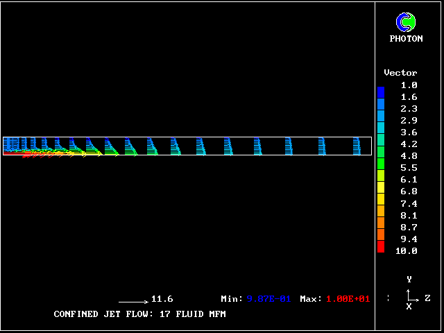
The geometrical grid is not too fine one, with 20 intervals along and 15 across duct.
/phoenics/d_polis/d_applic/mftm/vectors
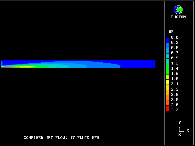
This is the distribution of the COMPUTED turbulence energy, /phoenics/d_polis/d_applic/mftm/ke
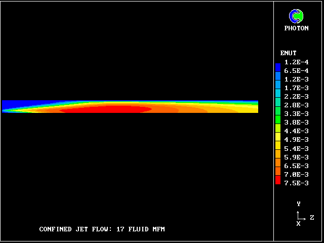
and this is the corresponding effective-viscosity distribution.
No surprises so far: all hydrodynamic turbulence quantities have come from standard K-epsilon model. /phoenics/d_polis/d_applic/mftm/enut
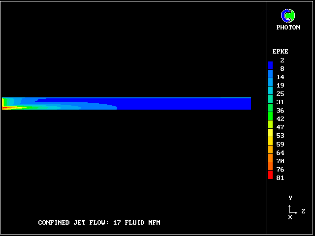
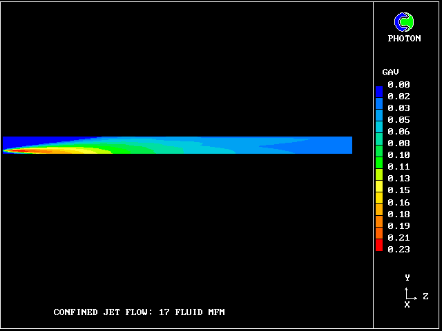
This quantity is closely related to multi-fluid approach for it represents the measure of the fluctuating motion of the turbulence, having dimensions of 1/sec.
It is this quantity, namely, epsilon divided by K, which is regarded as the micro-mixing rate.
/phoenics/d_polis/d_applic/mftm/epke
It is just as a model operating with transport equation for corresponding property would reveal ( see next picture );
but no transport equation of that kind is being computed !
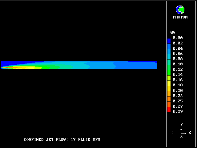
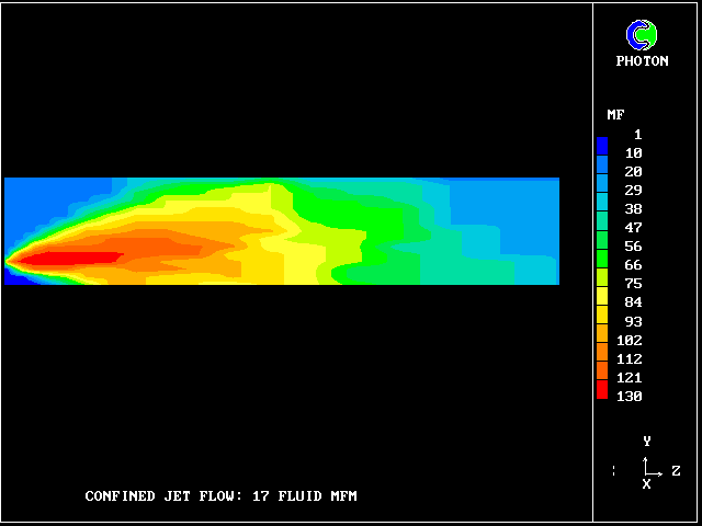
This is the concentration fluctuation distribution predicted by transport equation for the square of the fluctuating component.
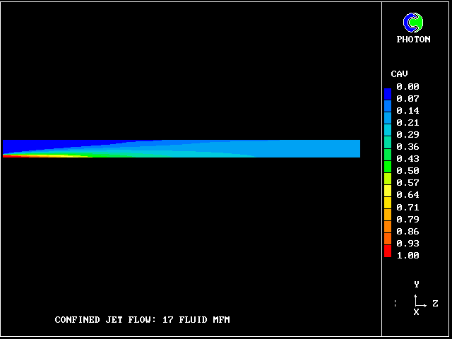
Here is the contour of population-average value of a central-jet fluid concentration. It is the same as the one calculated by conventional single fluid consideration.
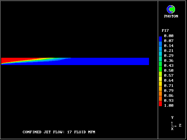
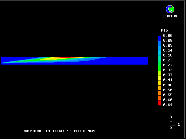
But how much surrounding fluid ( fluid 17 ) remains in its pure state? Only this.
Where has the rest gone?
What about pure central-jet fluid ( fluid 1 ) ?
It also occupies very little space.
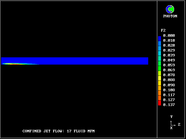
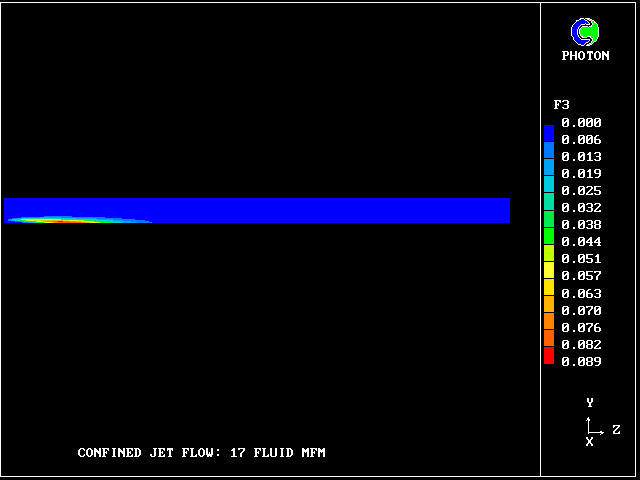
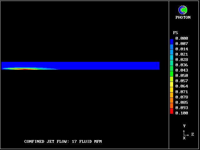
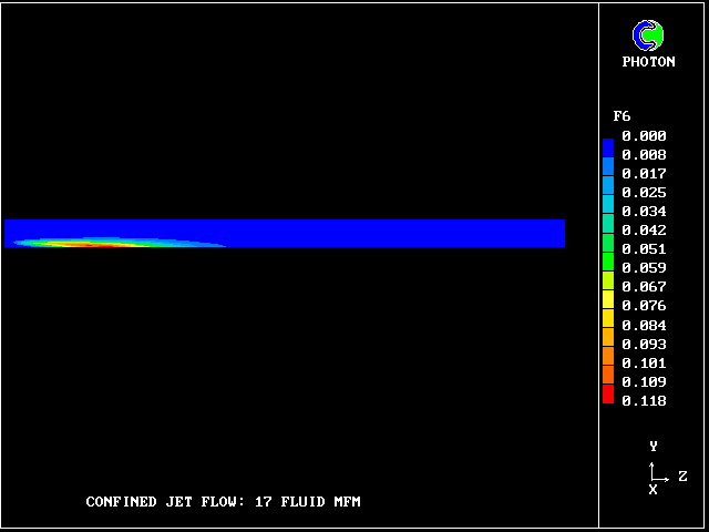
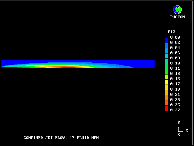
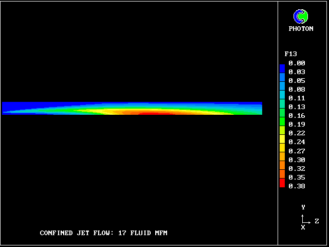
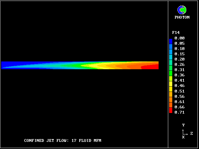
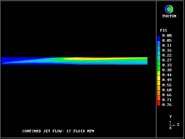
So what lies in between? 15 other fluids, variously intermingled. title5
The contours for fluid 2 The contours for fluid 3 The contours for fluid 4 The contours for fluid 5 The contours for fluid 6 The contours for fluid 7 The contours for fluid 8 The contours for fluid 9 The contours for fluid 10 The contours for fluid 11 The contours for fluid 12 The contours for fluid 13 The contours for fluid 14 The contours for fluid 15 The contours for fluid 16
ANOTHER MEANS OF REPRESENTING THE RESULTS
Here is a series of line-printer plots, showing the profiles of individual-fluid mass farctions along the symmetry axis of the duct.
All 17 fluid mass fractions will be shown.
Each is normalised, so as to have the same maximum ordinate.
PATCH(PROF1 ,PROFIL, 1, 1, 1, 1, 1, 20, 1, 1) PLOT(PROF1 ,F1 , 0.000E+00, 0.000E+00) MINVAL= 1.516E-05 MAXVAL= 1.000E+00
1.00 1111.+....+....+....+....+....+....+....+....+....+ 0.90 + + 0.80 + 1 + 0.70 + + 0.60 + + 0.50 + 1 + 0.40 + + 0.30 + 1 + 0.20 + + 0.10 + 1 + 0.00 +....+....+.1.1+.1..+1..1+..1.+.1..+1...1....1....1 0 .1 .2 .3 .4 .5 .6 .7 .8 .9 1.0 the abscissa is Z . min= 3.75E-03 max= 2.85E+00 PATCH(PROF2 ,PROFIL, 1, 1, 1, 1, 1, 20, 1, 1) PLOT(PROF2 ,F2 , 0.000E+00, 0.000E+00) MINVAL= 5.334E-08 MAXVAL= 1.165E-01
1.00 +....+1...+....+....+....+....+....+....+....+....+ 0.90 + + 0.80 + 1 + 0.70 + + 0.60 + 1 + 0.50 + + 0.40 + 1 + 0.30 + + 0.20 + 1 1 + 0.10 + 1 + 0.00 111..+....+....+.1..+1..1+..1.+.1..+1...1....1....1 0 .1 .2 .3 .4 .5 .6 .7 .8 .9 1.0 the abscissa is Z . min= 3.75E-03 max= 2.85E+00 PATCH(PROF3 ,PROFIL, 1, 1, 1, 1, 1, 20, 1, 1) PLOT(PROF3 ,F3 , 0.000E+00, 0.000E+00) MINVAL= 6.799E-08 MAXVAL= 7.866E-02
1.00 +....+.1..+....+....+....+....+....+....+....+....+ 0.90 + + 0.80 + 1 + 0.70 + 1 + 0.60 + + 0.50 + + 0.40 + + 0.30 + 1 1 + 0.20 + + 0.10 + 1 + 0.00 1111.+....+....+.1..+1..1+..1.+.1..+1...1....1....1 0 .1 .2 .3 .4 .5 .6 .7 .8 .9 1.0 the abscissa is Z . min= 3.75E-03 max= 2.85E+00 PATCH(PROF4 ,PROFIL, 1, 1, 1, 1, 1, 20, 1, 1) PLOT(PROF4 ,F4 , 0.000E+00, 0.000E+00) MINVAL= 3.416E-09 MAXVAL= 1.042E-01
1.00 +....+.1..+....+....+....+....+....+....+....+....+ 0.90 + + 0.80 + 1 + 0.70 + 1 + 0.60 + + 0.50 + + 0.40 + 1 + 0.30 + 1 + 0.20 + 1 + 0.10 + 1 1 + 0.00 111..+....+....+....+1..1+..1.+.1..+1...1....1....1 0 .1 .2 .3 .4 .5 .6 .7 .8 .9 1.0 the abscissa is Z . min= 3.75E-03 max= 2.85E+00 PATCH(PROF5 ,PROFIL, 1, 1, 1, 1, 1, 20, 1, 1) PLOT(PROF5 ,F5 , 0.000E+00, 0.000E+00) MINVAL= 1.045E-07 MAXVAL= 8.736E-02
1.00 +....+.1.1+....+....+....+....+....+....+....+....+ 0.90 + + 0.80 + + 0.70 + + 0.60 + 1 + 0.50 + 1 + 0.40 + + 0.30 + 1 + 0.20 + + 0.10 + 1 1 1 + 0.00 1111.+....+....+....+...1+..1.+.1..+1...1....1....1 0 .1 .2 .3 .4 .5 .6 .7 .8 .9 1.0 the abscissa is Z . min= 3.75E-03 max= 2.85E+00 PATCH(PROF6 ,PROFIL, 1, 1, 1, 1, 1, 20, 1, 1) PLOT(PROF6 ,F6 , 0.000E+00, 0.000E+00) MINVAL= 2.379E-10 MAXVAL= 1.079E-01
1.00 +....+...1+....+....+....+....+....+....+....+....+ 0.90 + 1 + 0.80 + 1 + 0.70 + + 0.60 + + 0.50 + 1 + 0.40 + 1 + 0.30 + + 0.20 + 1 + 0.10 + 1 1 + 0.00 1111.+....+....+....+...1+..1.+.1..+1...1....1....1 0 .1 .2 .3 .4 .5 .6 .7 .8 .9 1.0 the abscissa is Z . min= 3.75E-03 max= 2.85E+00 PATCH(PROF7 ,PROFIL, 1, 1, 1, 1, 1, 20, 1, 1) PLOT(PROF7 ,F7 , 0.000E+00, 0.000E+00) MINVAL= 2.811E-09 MAXVAL= 1.033E-01
1.00 +....+...1+.1..+....+....+....+....+....+....+....+ 0.90 + + 0.80 + + 0.70 + + 0.60 + 1 1 + 0.50 + + 0.40 + + 0.30 + 1 + 0.20 + 1 1 + 0.10 + 1 + 0.00 11111+....+....+....+....+..1.+.1..+1...1....1....1 0 .1 .2 .3 .4 .5 .6 .7 .8 .9 1.0 the abscissa is Z . min= 3.75E-03 max= 2.85E+00 PATCH(PROF8 ,PROFIL, 1, 1, 1, 1, 1, 20, 1, 1) PLOT(PROF8 ,F8 , 0.000E+00, 0.000E+00) MINVAL= 4.493E-09 MAXVAL= 1.237E-01
1.00 +....+....+.1..+....+....+....+....+....+....+....+ 0.90 + 1 + 0.80 + 1 + 0.70 + + 0.60 + + 0.50 + 1 1 + 0.40 + + 0.30 + 1 + 0.20 + 1 + 0.10 + 1 1 + 0.00 1111.+....+....+....+....+..1.+.1..+1...1....1....1 0 .1 .2 .3 .4 .5 .6 .7 .8 .9 1.0 the abscissa is Z . min= 3.75E-03 max= 2.85E+00 PATCH(PROF9 ,PROFIL, 1, 1, 1, 1, 1, 20, 1, 1) PLOT(PROF9 ,F9 , 0.000E+00, 0.000E+00) MINVAL= 1.329E-07 MAXVAL= 1.316E-01
1.00 +....+....+.1.1+....+....+....+....+....+....+....+ 0.90 + + 0.80 + + 0.70 + 1 1 + 0.60 + + 0.50 + + 0.40 + 1 + 0.30 + 1 + 0.20 + 1 + 0.10 + 1 1 + 0.00 11111+....+....+....+....+....+.1..+1...1....1....1 0 .1 .2 .3 .4 .5 .6 .7 .8 .9 1.0 the abscissa is Z . min= 3.75E-03 max= 2.85E+00 PATCH(PROF10 ,PROFIL, 1, 1, 1, 1, 1, 20, 1, 1) PLOT(PROF10 ,F10 , 0.000E+00, 0.000E+00) MINVAL= 3.950E-11 MAXVAL= 1.588E-01
1.00 +....+....+...1+....+....+....+....+....+....+....+ 0.90 + 1 + 0.80 + 1 + 0.70 + + 0.60 + 1 + 0.50 + 1 + 0.40 + 1 + 0.30 + + 0.20 + 1 1 + 0.10 + 1 1 + 0.00 11111+....+....+....+....+....+....+1...1....1....1 0 .1 .2 .3 .4 .5 .6 .7 .8 .9 1.0 the abscissa is Z . min= 3.75E-03 max= 2.85E+00 PATCH(PROF11 ,PROFIL, 1, 1, 1, 1, 1, 20, 1, 1) PLOT(PROF11 ,F11 , 0.000E+00, 0.000E+00) MINVAL= 1.159E-10 MAXVAL= 1.891E-01
1.00 +....+....+....+.1..+....+....+....+....+....+....+ 0.90 + 1 + 0.80 + 1 + 0.70 + 1 + 0.60 + + 0.50 + 1 + 0.40 + 1 + 0.30 + 1 + 0.20 + 1 + 0.10 + 1 1 1 + 0.00 11111+1...+....+....+....+....+....+....+....1....1 0 .1 .2 .3 .4 .5 .6 .7 .8 .9 1.0 the abscissa is Z . min= 3.75E-03 max= 2.85E+00 PATCH(PROF12 ,PROFIL, 1, 1, 1, 1, 1, 20, 1, 1) PLOT(PROF12 ,F12 , 0.000E+00, 0.000E+00) MINVAL= 4.136E-10 MAXVAL= 2.312E-01
1.00 +....+....+....+....+1..1+....+....+....+....+....+ 0.90 + + 0.80 + 1 1 + 0.70 + + 0.60 + + 0.50 + 1 1 + 0.40 + + 0.30 + 1 1 + 0.20 + 1 1 + 0.10 + 1 1 1 0.00 11111+1...+....+....+....+....+....+....+....+....+ 0 .1 .2 .3 .4 .5 .6 .7 .8 .9 1.0 the abscissa is Z . min= 3.75E-03 max= 2.85E+00 PATCH(PROF13 ,PROFIL, 1, 1, 1, 1, 1, 20, 1, 1) PLOT(PROF13 ,F13 , 0.000E+00, 0.000E+00) MINVAL= 2.352E-09 MAXVAL= 3.281E-01
1.00 +....+....+....+....+....+..1.+.1..+....+....+....+ 0.90 + 1 + 0.80 + 1 + 0.70 + 1 + 0.60 + 1 1 + 0.50 + + 0.40 + 1 1 0.30 + + 0.20 + 1 + 0.10 + 1 1 + 0.00 11111+11..+....+....+....+....+....+....+....+....+ 0 .1 .2 .3 .4 .5 .6 .7 .8 .9 1.0 the abscissa is Z . min= 3.75E-03 max= 2.85E+00 PATCH(PROF14 ,PROFIL, 1, 1, 1, 1, 1, 20, 1, 1) PLOT(PROF14 ,F14 , 0.000E+00, 0.000E+00) MINVAL= 6.147E-10 MAXVAL= 6.604E-01
1.00 +....+....+....+....+....+....+....+....+....+....1 0.90 + 1 + 0.80 + 1 + 0.70 + 1 + 0.60 + + 0.50 + 1 + 0.40 + 1 + 0.30 + 1 + 0.20 + 1 + 0.10 + 1 1 + 0.00 11111+11.1+.1..+....+....+....+....+....+....+....+ 0 .1 .2 .3 .4 .5 .6 .7 .8 .9 1.0 the abscissa is Z . min= 3.75E-03 max= 2.85E+00 PATCH(PROF15 ,PROFIL, 1, 1, 1, 1, 1, 20, 1, 1) PLOT(PROF15 ,F15 , 0.000E+00, 0.000E+00) MINVAL= 2.323E-09 MAXVAL= 1.716E-01
1.00 +....+....+....+....+....+....+....+....+....+....1 0.90 + 1 + 0.80 + 1 + 0.70 + 1 + 0.60 + 1 + 0.50 + 1 + 0.40 + 1 + 0.30 + 1 + 0.20 + 1 + 0.10 + 1 1 + 0.00 11111+11.1+....+....+....+....+....+....+....+....+ 0 .1 .2 .3 .4 .5 .6 .7 .8 .9 1.0 the abscissa is Z . min= 3.75E-03 max= 2.85E+00 PATCH(PROF16 ,PROFIL, 1, 1, 1, 1, 1, 20, 1, 1) PLOT(PROF16 ,F16 , 0.000E+00, 0.000E+00) MINVAL= 9.501E-09 MAXVAL= 1.822E-02
1.00 +....+....+....+....+...1+..1.+....+....+....+....+ 0.90 + 1 1 + 0.80 + + 0.70 + 1 1 + 0.60 + + 0.50 + 1 + 0.40 + 1 1 + 0.30 + 1 1 + 0.20 + 11 1 0.10 + 1 + 0.00 1111.+....+....+....+....+....+....+....+....+....+ 0 .1 .2 .3 .4 .5 .6 .7 .8 .9 1.0 the abscissa is Z . min= 3.75E-03 max= 2.85E+00 PATCH(PROF17 ,PROFIL, 1, 1, 1, 1, 1, 20, 1, 1) PLOT(PROF17 ,F17 , 0.000E+00, 0.000E+00) MINVAL= 1.115E-07 MAXVAL= 5.479E-03
1.00 +....+....+....+.1..+1...+....+....+....+....+....+ 0.90 + 1 1 + 0.80 + 1 + 0.70 + 1 + 0.60 + 1 + 0.50 + 1 + 0.40 + 1 1 + 0.30 + + 0.20 + 1 1 1 + 0.10 + 1 1 0.00 1111.+....+....+....+....+....+....+....+....+....+ 0 .1 .2 .3 .4 .5 .6 .7 .8 .9 1.0 the abscissa is Z . min= 3.75E-03 max= 2.85E+00 YET ANOTHER MEANS OF REPRESENTING THE RESULTS
Any observer of the sky can see the patchiness of its cloud cover; and tongues of smoke interspersed with clear-air fragments are evident in every back-yard bonfire.
To make visible the intermittency and fragmentariness of turbulence phenomena in question the marker technique can be used as follows.
Individual fluids markers are introduced : M1 = 1 stands for 1.0 fluid mass fraction greater than 0.01 M2 = 2 stands for 15/16 fluid mass fraction greater than 0.01 M3 = 3 stands for 14/16 fluid mass fraction greater than 0.01 and so on.
Then the total marker can be calculated as the cell-wise sum of all individual markers so that: MF = 6 marks the region occupied, say, by 1.0, 15/16 and 14/16 fluids of mass fraction greater than 0.01.
Here is the contours of the total fluid marker showing the fragmentariness of the concentration distributions.
/phoenics/d_polis/d_applic/mftm/frag
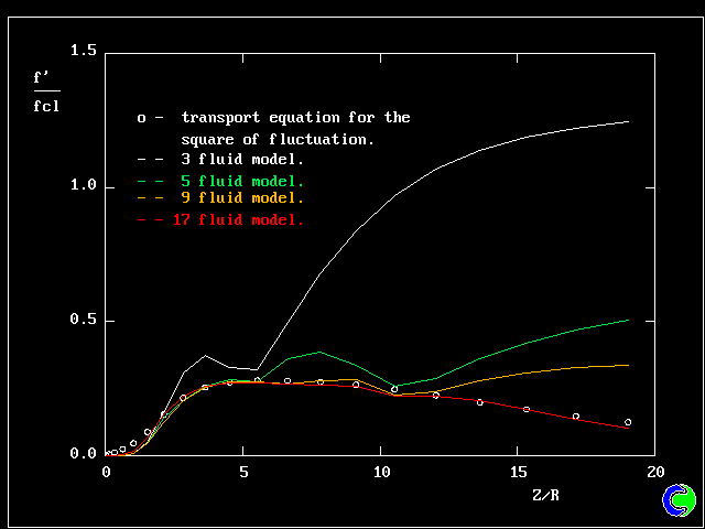
Fluid-population-grid-refinement studies requires detailed attention. We must find out how fine a grid is needed for the accuracy to be reasonable enough for practical purposes.
There will now be presented a series of graphs, all for the same boundary conditions, the same value of mixing constant and the same monitoring directions.
Specifically the models will have 3, 5, 9 and 17 fluids with uniformly distributed fluid attribute. It was found that further refinement of fluid population grid has little influence on the computational results.
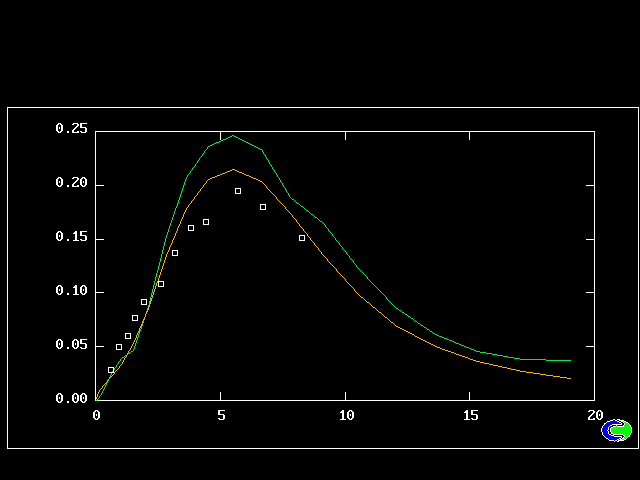
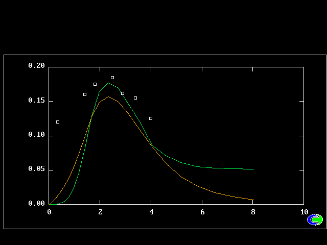
The next picture shows the variations with axial distance the averaged concentration fluctuations at the axis. In each case, it is normalised by the local concentration of the central-jet fluid and axial distance is normalised by duct radius.
The full curves represent multi-fluid predictions and the points are the computations of the transport equations for the square of the concentration fluctuations.
/phoenics/d_polis/d_applic/mftm/fr
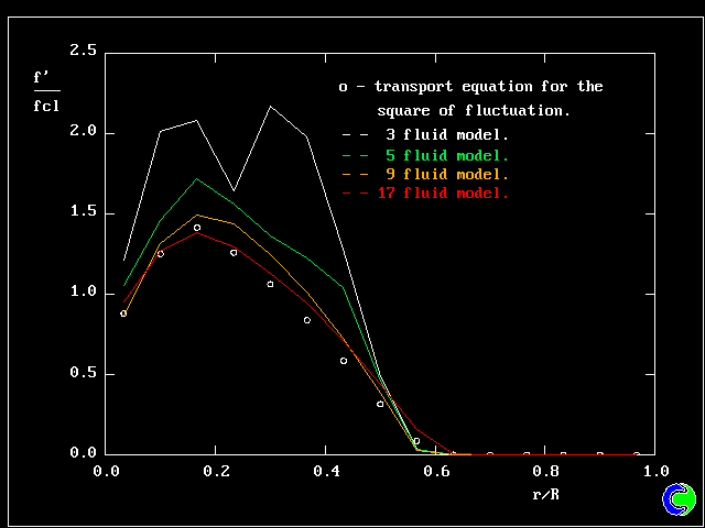
The radial variation of the averaged concentration fluctuations are shown in the next picture. The full lines are multi-fluid predictions and the points are the computations of the transport equations for the square of the concentration fluctuations.
The ordinates represent values of the averaged concentration fluctuations normalised by its value at the axis of symmetry, and the abscissae is radial distance normalised by the duct radius.
Fair agreement is seen between multi-fluid predictions and transport equation for turbulence quantity for finest ( not too much ) fluid-population grid used for all above calculations.
/phoenics/d_polis/d_applic/mftm/fi
In the next two panels the results of numerical computations are compared with experimental measurements of concentration fluctuations extracted from the work of Elgobashi et all.
These comparisons show that single constant of MFM provides fair agreement between calculations and experiment for the cases when a region of recirculation is appeared downstream of the inlet plane.
This plot displays the predicted and measured axial variations of normalised averaged concentration fluctuations for Craya-Curtet number equals to 0.875. Points are the experiments of Torrest and Ranz.
Green line - MFM prediction Yellow line - transport equation /phoenics/d_polis/d_applic/mftm/0012 This plot displays the predicted and measured axial variations of normalised averaged concentration fluctuations for Craya-Curtet number equals to 0.345. Points are the experiments of Becker, Hottel and Williams;
Green line - MFM prediction Yellow line - transport equation /phoenics/d_polis/d_applic/mftm/0016
Overall, it can be said that fair agreement between MFM predictions and experiments is observed.
The axial location of maximum concentration fluctuations is well reproduced.
MFM is slightly over-predicted the actual values in comparison with transport equation calculations for Craya-Curtet number equals to 0.875.
For the flow with Craya-Curtet number of 0.345, it seems that the inlet concentration fluctuations in experiment were not negligible. It results in under-prediction of both transport equation model and MFM which treat the flow to be well stirred at the inlet plane with no concentration fluctuations whatsoever.
8. Conclusion --------------
The use of multi-fluid approach together with K-epsilon turbulence model for hydrodynamics has been found to give satisfactory prediction for the concentration fluctuations in confined jet flow.
The number of tests performed have proved the self-consistency and conservativeness of the model formulation, the correct behavoir of the equation system under the influences of micro-mixing constant and of the "population grid".
It has been established, that refining the population grid (ie increasing the number of fluids) does indeed lead to a unique solution, and though grid refinement from 3 to 5 is not enough for grid-independent results to be attained; but as few as 17 fluids give acceptable accuracy.
Concentration fluctuation results have provided further validity of the analysis put forward by Spalding. For the present case, where k-epsilon model is used for simulating the hydrodynamics, there is only one constant needed by the model, namely that which relates the "fluid-coupling" rate to epsilon/k; and the best value is found to be 5.0.
The ability of the model to reproduce the results of the solution of transport equations for turbulence quantities, as well as experimental observations is especially gratifying.
More reliable experimental data are still needed for a more extensive validation of the multy-fluid model. However, it seems that sufficient confidence has already been generated.
9. References ------------- DB Spalding (1995) "Models of turbulent combustion" Proc. 2nd Colloquium on Process Simulation, pp 1-15 Helsinki University of Technology, Espoo, Finland
DB Spalding (1995) "Multi-fluid models of Turbulence", European PHOENICS User Conference, Trento, Italy
DB Spalding (1996) "Older and newer approaches to the numerical modelling of turbulent combustion". Keynote address at 3rd International Conference on COMPUTERS IN RECIPROCATING ENGINES AND GAS TURBINES, 9-10 January, 1996, IMechE, London
SE Elgobashi, WM Pun and DB Spalding (1977) " Concentration fluctuation in isothermal turbulent confined coaxial jets". Chemical Engineering Science, v. 32, pp. 161-166
Appendix. Q1 file for 17 fluid model
TALK=f;RUN( 1, 1);VDU=VGAMOUSE
TEXT(CONFINED JET FLOW: 17 FLUID MFM ------------------------------- REAL(HIN,GMIXL,CLEN,WIDTH,WIN1,WIN2,REYNO,WD2) REAL(TKEIN1,EPIN1,TKEIN2,EPIN2) INTEGER(IYJ);IYJ=3 REYNO=1.E6;WIDTH=0.3;HIN=1. WIN1=10.;WIN2=2.0
CARTES=F;XULAST=0.1 NY=15;WD2=0.5*WIDTH;GRDPWR(Y,NY,WD2,1.0) NZ=20;CLEN=20.*WD2;GRDPWR(Z,NZ,CLEN,2.0)
** H1 - single fluid concentration variable; g - square of concentration fluctuation; SOLVE(P1,W1,V1,H1,G) ** GENG - production for the square of concentration fluctuation STORE(ENUT,LEN1,GEN1,EPKE,GENG)
SOLUTN(P1,Y,Y,Y,N,N,N) TURMOD(KEMODL)
TERMS(H1,N,Y,Y,Y,Y,Y) TERMS( G,N,Y,Y,Y,Y,Y)
RHO1=1.0;ENUL=WIN1*WIDTH/REYNO PRT(H1)= 0.86;PRNDTL(H1)= 0.71 PRT(G) = 0.7 ;PRNDTL(G) = 0.7
GROUP 11. Initialization of variable or porosity fields FIINIT(W1)=0.5*(WIN1+WIN2);FIINIT(H1)=HIN FIINIT(LEN1)=0.1*YVLAST FIINIT(ENUT)=0.01*WIN1*YVLAST ** TKEIN = 0.25*WIN1*WIN1*FRIC where FRIC=0.018 AT REYNO=1.E5 TKEIN1=0.25*WIN1*WIN1*0.018 TKEIN2=0.25*WIN2*WIN2*0.018 FIINIT(KE)=0.5*(TKEIN1+TKEIN2) ** EPIN = 0.1643*KIN**1.5/LMIX where LMIX=0.045*WIDTH GMIXL=0.011*WD2 EPIN2=TKEIN2**1.5/GMIXL*0.1643 EPIN1=TKEIN1**1.5/GMIXL*0.1643 FIINIT(EP)=0.5*(EPIN1+EPIN2) FIINIT(P1)=1.3E-4
GROUP 13. Boundary conditions and special sources ** Inlet Boundaries INLET(IN1,LOW,1,1,1,IYJ,1,1,1,1) VALUE(IN1,P1 , WIN1) VALUE(IN1,W1 , WIN1) VALUE(IN1,H1 , 1.0) VALUE(IN1,KE , TKEIN1) VALUE(IN1,EP , EPIN1) VALUE(IN1,G , 0.0)
INLET(IN2,LOW,1,1,IYJ+1,NY,1,1,1,1) VALUE(IN2,P1, WIN2) VALUE(IN2,W1, WIN2) VALUE(IN2,H1, 0.0) VALUE(IN2,KE, TKEIN2) VALUE(IN2,EP, EPIN2) VALUE(IN2,G , 0.0)
**Outlet boundary PATCH(OUTLET,HIGH,1,NX,1,NY,NZ,NZ,1,1) COVAL(OUTLET,P1,1.0e05,0.0) COVAL(OUTLET,W1,ONLYMS,0.0);COVAL(OUTLET,V1,ONLYMS,0.0) COVAL(OUTLET,KE,ONLYMS,0.0);COVAL(OUTLET,EP,ONLYMS,0.0)
**North-Wall boundary (generalised wall functions)
WALL (WFNN,NORTH,1,NX,NY,NY,1,NZ,1,1)
**Source term for g
PATCH(SORG,VOLUME,1,NX,1,NY,1,NZ,1,1)
LSWEEP=500; RESFAC=0.01
LITHYD=10 ; KELIN=3
RELAX(P1,LINRLX,0.25)
RELAX(V1,FALSDT,0.025)
RELAX(W1,FALSDT,0.025)
RELAX(KE,FALSDT,0.025)
RELAX(EP,FALSDT,0.025)
RELAX(G,FALSDT ,0.025)
WALPRN=T
OUTPUT(KE,Y,Y,Y,Y,Y,Y);OUTPUT(H1,Y,Y,Y,Y,Y,Y)
IZMON=NZ-1;IYMON=NY-1;UWATCH=T
NPLT=1;NZPRIN=1
NYPRIN=1;IYPRF=1;IYPRL=30
NAMSAT=MOSG
** Number of fluids in population
INTEGER(NFLUIDS); NFLUIDS=17
** Micro-mixing constant
REAL(MMC); MMC = 5.0 ; RG(1) = MMC
** Solve for fluid mass fractions F1, F2, ..., F17
DO II=1,NFLUIDS
SOLVE(F:II:);TERMS(F:II:,N,Y,y,y,y,y)
PRT(F:II:)= 0.86;PRNDTL(F:II:)= 0.71
RELAX(F:II:,linrlx,0.15)
VARMIN(F:II:)=0.0;VARMAX(F:II:)=1.0
PATCH(PROF:II:,PROFIL,1,1,1,1,1,20,1,1)
PLOT(PROF:II:,F:II:,0.000E+00, 0.000E+00)
ENDDO
** Fluid population boundary conditions
DO II=1,NFLUIDS
VALUE(IN1,F:II:,0.0);VALUE(IN2,F:II:,0.0)
ENDDO
VALUE(IN1,F1 , 1.0); VALUE(IN2,F:NFLUIDS:, 1.0)
** Coupling/splitting rates
PATCH(MIX,PHASEM,1,NX,1,NY,1,NZ,1,1)
* Fluid 1
* Fluid 5
* Fluid 9
* Fluid 12
* Fluid 15
** Output calculations
CAV - averaged concentration of central jet fluid;
GAV - averaged concentration fluctuation;
GF - averaged concentration fluctuation normalised
by local averaged concentration of central jet fluid.
MAS - sum of fluid mass fractions;
STORE(CAV,MAS,GAV,GF)
FIINIT(GF)=0.0
STOP
--------------- The END --------------------