Iterative solution procedures are said to be converging when the changes in solved-for values become smaller with each iteration and are finally negligible. Convergence is thus what one wishes all flow-simulating computations to exhibit.
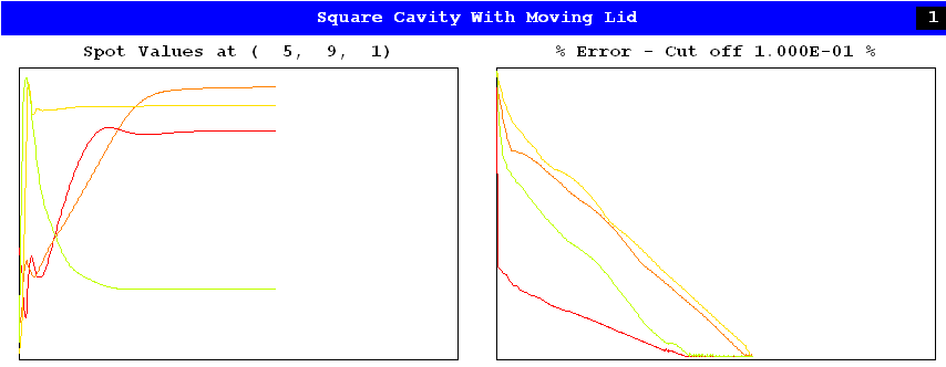
The following picture illustrates convergence. They are generated by PHOENICS Input-File-Library Case 249, concerned with laminar flow and heat in a square cavity with a moving lid.
That these curves become horizontal as the abscissa increases proves that indeed the changes have become very small; for the abscissa measures the iteration (called 'sweep') number.
The curves on the right represent the (logarithms of the) sums of the absolute residuals of each variable. These fall satisfactorily to the user-set target value; whereupon the computation terminates.
Not all computations converge so rapidly, as the next picture shows. It refers to the same flow situation, that of library case 249; but CONWIZ, which controls the built-in convergence promoter of PHOENICS, has been set to F rather than T.
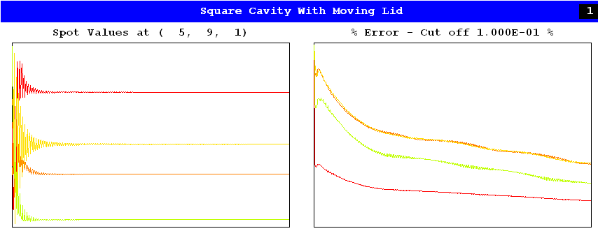
Convergence does still occur, but more slowly; and the residuals do not fall far enough to terminate the calculation.
Convergence has occurred because the default values of the relevant relaxation parameters happened to suffice. Inspection of the RESULT file shows these to be:
 Group 17. Relaxation
 RELAX(P1,LINRLX,1.)
 RELAX(U1,FALSDT,1.)
 RELAX(V1,FALSDT,1.)
 RELAX(H1,FALSDT,1.0E+09)
If now the velocity-related defaults are over-written by inserting in the Q1 file:
 RELAX(U1,FALSDT,1.E6)
 RELAX(V1,FALSDT,1.E6)
the following picture is generated:
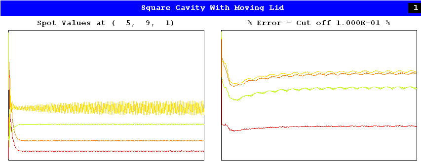
This run did not converge; but nor did it diverge. Divergence is shown however by the following picture which resulted when the even more unsuitable settings:
 Group 17. Relaxation
 RELAX(P1,LINRLX,2.0)
 RELAX(U1,FALSDT,1.E6)
 RELAX(V1,FALSDT,1.E6)
were made.
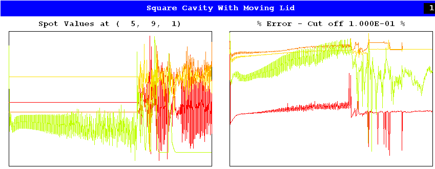
The divergence of the last example was contrived deliberately by (as it is said) over- relaxing the pressure variable, P1, through choosing a value of its linear-relaxation factor in excess of 1.0.
Unfortunately divergence can appear in practice when the relaxation settings are far from perverse; indeed even when they are the best that the user knows how to select.
The rest of this article is devoted to providing advice on what is then to be done.
The following discussion is organized under the headings:
A common error of inexperienced users is to set very small values of the false time step, e.g. 1.0e-3 sec for the velocity. They then find that the oscillations which have alarmed them disappear; and they are comforted by the apparently smooth progress of the solution procedure, not recognising that it is proceeding so slowly that an intolerably large number of sweeps will be needed to attain the true solution.
For a wind-farm simulation for example, in which a 10 km width and a 10 km/sec wind imply that effects take 1000 sec to be convected across the domain, even a 1.0 sec false time step imposes a severe delay on the attainment of the correct solution.
The default value of the dveldp relaxation parameters is 0.5; but users can use change these by inserting into the Q1 statements such as:
SPEDAT(RLXFAC,RLXDU1,R,0.25)
SPEDAT(RLXFAC,RLXDV1,R,0.25)
in order to slow down the sweep-to-sweep changes in values.
It is especially important for flow-over-natural-terrain problems; for steep gradients of just one part of the ground surface may suffice to cause divergence if GCV is left at its default value, namely F.
An example is this:
The setting of the PIL variables VARMIN and VARMIX can prevent this from occurring.
Of the two modes of using these variables, that which sets limits to the increments of variables is the preferable. Thus, if VARMIN(temperature) is set to -1.e-11 (to trigger that mode) and VARMAX(temperature) to 10.0 deg Celsius, the above-mentioned second-sweep divergence will simply be unable to occur.
Less drastic but still troublesome failure to converge can usually be controllled in this way.
If one knew the solutions to the equations at the start, and could insert the corresponding variable-field values as initial guesses, convergence would be immediate. Of course, the solutions never are known; however, if initial guesses can be made which are close to these solutions, convergence is likely to be rapid.
It is therefore usually worthwhile to set values of the initial fields, by way of FIINIT, which are as close as possible to the expected average values of the solutions. It is possible to do even better, if the PATCH and INIT commands are used; for these permit linearly-varying values (and indeed more complicated piece-wise linear distributions) to be inserted rather easily. Even more powerful is In-Form's (initial of variable_name is formula) command.
How far to go in this direction should be determined by reference to the man-time cost of determining and introducing suitable initial values and of the computer-time cost that is thereby saved.
A means of saving computer time that requires very little man-time, once the system has been set up, is to employ the SPINTO facility. This launches a series of runs, on increasingly finer grids. Each run uses as its initial field values obtained by interpolation from the output of the previous run.
It often occurs that convergence proceeds smoothly, but not fast enough. In order to establish whether acceleration may be possible, the cause of slow convergence should first be sought among the following:-
How can one determine whether one of the above is contributing to excessive computer charges? By changing the relevant settings and observing what happens. Every reduction in the amount of under- relaxation, even an enlargement in time step, is to be welcomed, provided that it does not on the one hand lead to divergence or on the other entail a significant falling off in numerical accuracy.
It is recommended that only the second-phase volume-fraction equation is solved when the two phases coexist everywhere in finite proportions, e.g. the volume fraction of one of the phases never falls below 0.001. The following PIL instruction:
SOLUTN(R1,Y,N,...); SOLUTN(R2,Y,Y,...),
causes EARTH to solve for R2 and to calculate R1 as 1-R2. In addition to being more economical than solving for R1 and R2, this practice has proved to give faster convergence in several 2-phase simulations.
When the phase volume fractions do not coexist everywhere in finite proportions, it is necessary to solve R1 and R2, by way of the settings:
SOLUTN(R1,Y,Y,...); SOLUTN(R2,Y,Y,...).
Were R2 alone solved in this situation, loss of accuracy would occur in the calculation of R1 from 1-R2 in those location in which R2 is close to unity.
There are other measures which can be taken at the SATELLITE level in order to reduce computer time. One important one is to change the choice of solution procedure in the light of the considerations discussed in Section 5.4. The point-by-point procedure should be used for the velocity components and volume fractions when the diffusion terms are of little importance; but it should definitely not be used otherwise.
Different velocity components may need different solution procedures. For example, a boundary-layer flow in which z is the predominant flow direction is best handled with point- by-point solution for u and v, but slab-wise solution for w. The reason is that w is strongly influenced by viscosity in these circumstances,whereas u and v are not.
In some fluid-flow simulations, it is best to use the TERMS command in order to switch off the viscous terms entirely. More surprisingly, perhaps, it is sometimes permissible to switch off the convection terms as well. For example, when the flow takes place in a porous medium such as EARTH or sand, the only important terms are the pressure gradient and the resistance exerted by the medium; so there is no point in computing terms which are negligible. The Encyclopaedia entry, Darcy, explains how to activate this feature.
A number of other devices e.g. ADDDIF, GALA, ZDIFAC, NEWRH1 etc. are available for solution control and economy. These are in Group 8; they are described in the Encyclopaedia.
Finally, attention is drawn once more to the possibility of varying the starting-time and the frequency of updating of the various dependent variables, and for that matter of the auxiliary variables as well. PHOENICS possesses many devices for effecting such variations, which you are advised to explore.
The guiding principle should be this: quantities which both influence and are influenced by the velocity (or other dominant-variable) field should be updated frequently throughout the computation; those which influence but are not influenced should be set at the beginning and never updated; and those which are influenced but do not influence should be updated only at the end.