Since boundary conditions are, in PHOENICS, represented by way of sources, they too are the subject of the present discussion.
A simple example is provided by library case 105, where indeed the old (PIL) and the new (In-Form) ways of setting sources are compared, just as was earlier done in respect of initial values.
For a reminder of the significance of PIL's COVAL command, click here.
In-Form statements containing the 'source' keyword commonly contain pre-formula and post-formula qualifiers. In the case just referred to:
Here it may be remarked that linearization was activated in the pre-In-Form (i.e. COVAL-command) formulation by the user's provision of separate CO and VAL arguments; and, if a truly non-linear source had been required, the user would have been at a loss.
In-Form will however of its own accord linearize
non-linear sources also, for example:
(SOURCE of H1 at WHOLE is 1.e4*(2.0-h1)^3 with LINE)
the non-linearity being caused by the '^3' insertion.
It does so however only when the source decreases with increase of the solved-for variable (i.e. H1 in this case); for, otherwise, numerical instability might occur.
However, for many problems, it is as easy (or easier) to provide formulae for the 'coefficient' and 'value' directly; then the automatic linearizing procedure is not necessary.
For such cases, In-Form provides the COVAL function, the two arguments of which are the formulae for the coefficient (i.e. CO) and the value (i.e. VAL). The main features of this function are:-
(SOURCE of Var_Name at Patch_Name is
COVAL(Coef_Formula,Value_Formula) with Flags)
where:
Coef_Formula and Value_Formula
are formulae in which the words:
FIXFLU, FIXVAL, FIXP, ONLYMS, OPPVAL and SAME
can be used just as in the PIL command, COVAL .
(SOURCE of H1 at X1 is COVAL(FIXV,0.0))
(SOURCE of H1 at WHOLE is COVAL(1.e4,2.0))
Numerous examples of the various means of setting sources and boundary conditions will be found in the following sections, which are organized in accordance with the means of localization employed, namely:
The option 'with FIXF' is rarely encountered in an In-Form SOURCE statement because it is the default option, meaning 'do not linearise'; however, when the COVAL function is in use, FIXF often appears as the first argument of that function, as for example in library case 747.
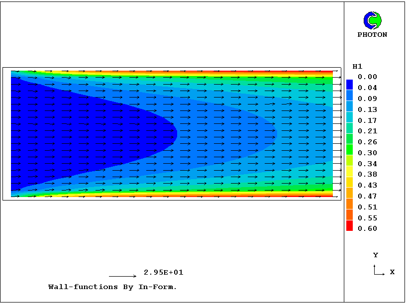
The resulting enthalpy distribution in the duct is shown here.
Inspection of the relevant statements in the Q1 shows that:
In case 748, the 'In-Form' way of setting wall conditions is compared with the 'PIL COVAL' way by using them for opposite walls of a plane-walled duct.
The solution should be symmetrical, as indeed it is.
The COVAL function is not illustrated in this case; but it could have been used.
This signifies, as will be easily understood by those who recall that ONLYMS can also be the third argument of a PIL COVAL statement, that the enthalpy flux consists of the enthalpy defined by the formula (here TWALLMAX*0.2) times the mass flux.
Although the flow is two-dimensional, NZ has been set to 2, in order that one means of setting the sources can be used for IZ=1 and another for IZ=2.
There are three such sources, two for wall boundary conditions and the third within the domain.
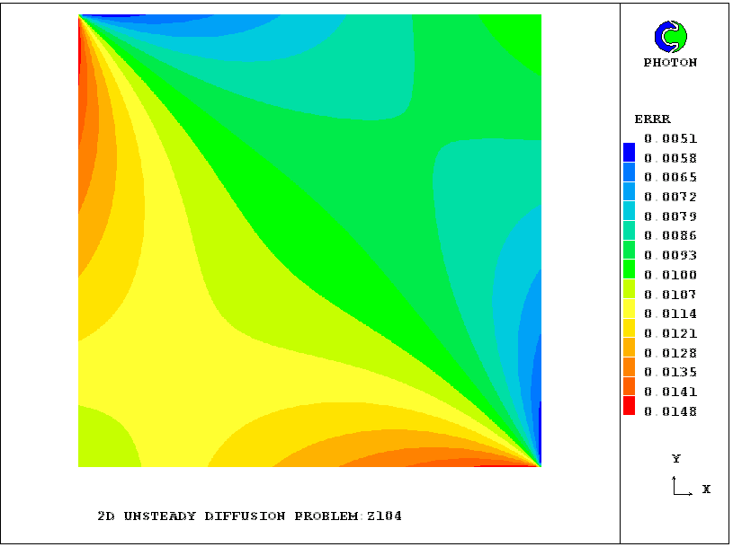
Also computed, and given values by way of an In-Form source with fixval, is the variable named ERRR which represent the difference between the two solutions, a contour plot of which is shown here.
It is interesting to observe that the maximum and minimum errors (of the order of 1%) are to be found near the north-west and south-east corners.
PATCH(INL,WEST,1,1,1,NY,1,1,1,1)
(SOURCE of P1 at Patch_Name is Input_mass_flow_formula)
(SOURCE of P1 at INL is RHO1*VELIN)
where VELIN is input velocity, and RHO1 the density.
An example can be found in library case 746 which is concerned especially with In-Form-based boundary conditions.
COVAL(INL,P1,FIXFLU,RHO1*VELIN)
to which the In-Form statement is not particularly superior.
For example a parabolic distribution of mass flow across the entrance to a channel can be prescribed via:
(SOURCE of P1 at INL is RHO1*VELMAX*(1.-(2.*YG/YVLAST-1)^2))
where:
YG is the distance of the grid point from the south wall, YVLAST the distance from the south wall to the north and VELMAX is the Maximum velocity, as is to be found in library cases 745 and 747 .
Separate (parabolic-mode) PHOENICS studies of the plume have shown that the plume has an approximately sinusoidal velocity profile; and it is therefore this which must be provided as an input to the (elliptic) upper-layer calculation.
The relevant lines are:
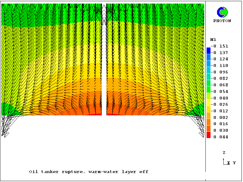
patch(leak,low,1,1,1,12,1,1,1,1)
(source of p1 at leak is 1000*0.03*sin((532-yg)/338.7) with
fixflu)
from which it can be deduced that the half-width of the sine curve is 532 meters.
The resulting w1 contours and velocity vectors near the base of the layer can be seen here.
The contours show that the fluid entering from below quickly changes its direction to horizontal and then downward, no doubt because of the influence of the density gradients.
This case will be referred to again under the heading of 'momentum sources'.
The injection rate increases linearly with distance along the duct.
In each case, two Z-slabs are employed solely in order that alternative means of setting In-Form sources, for example with or without the COVAL function, produce identical results.
Case 746 is the simplest; for the 'formula' of the In-Form source statement is simply: 'VELIN with ONLYMS', the latter condition signifying that the momentum flux into each cell equals VELIN times the mass flow per unit area.
The 'with ONLYMS' condition is identical in its action to that of ONLYMS as the third argument of a PIL COVAL command.
Had the condition not been supplied, the formula would have
had to be written as:
RHO1*VELIN^2 .
Similar remarks are appropriate about cases 745 and 747.
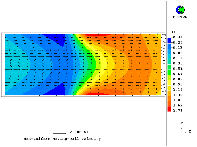
The COVAL commmand of PIL could express this condition perfectly well; but this is not true of case 745, in which the walls are moving at velocities which are proportional to XU, the distance along the duct. For this, In-Form's capabilities are needed.
Inspection of the two lines:
(source of p1 at leak is 1000*0.03*sin((532-yg)/338.7) with fixflu)
(source of w1 at leak is 0.03*sin((532-yg)/338.7) with onlyms)
reveals that the 'formula' in the second, which represents the momentum source, is the same as that in the first, apart from the absence of the 1000.0 which represents the density.
Coupled with the condition 'with ONLYMS', this entails that the
momentum flux per unit area is:
density * velocity ** 2 .
which is what is required.
PATCH(ALL,CELL,1,NX,1,NY,1,NZ,1,LSTEP)
(SOURCE of U1 at ALL is 1.E5*(VEL*(YIC-YG)-U1) with IMAT>=PAD!LINE)
(SOURCE of V1 at ALL is 1.E5*(VEL*(XG-XIC)-V1) with IMAT>=PAD!LINE)
which signify that, over the patch named ALL (which extends over the whole
domain), the sources are proportional
to the difference between the prevailing velocity at the point and the
position-dependent quantities:
VEL*(YIC-YG) and VEL*(XG-XIC).
The constant multiplying the velocity differences has been made large, so as to causes U1 and V1 to be close to the desired values.
The time-dependence is brought about by clever use of the STORED keyword, which, being placed in a DO loop in the Q1 file, provides a different distribution of IMAT at the start of each times step.
This is not the most economical method of simulating a moving object (see section 8 for better ones); but it well illustrates the power of well-chosen In-Form statements.
The condition IMAT>=PAD, signifies that the source is to be applied only to those cells for which the PRPS-value, IMAT, is greater than or equal to PAD, the material index of the paddle, which happens to be 100., which is greater than the 67.0 (signifying water) which prevails elsewhwere in the domain.
Following the delimiter is a second condition, namely "LINE", which is an abbreviation of "LINEARISED".
This is an instruction which requires that the source is introduced in the linearised manner which ensures that it becomes zero when the velocity equals the desired value.
Without this condition, the source would have been created in the "fixed-flux" manner, which, in COVAL statements, is specified by setting FIXFLU as the third argument.
In the formulae used, VABS stand for the absolute velocity at the centre of the scalar cells, 1000. for the presumed fluid velocity and 0.003 for the friction factor which it is desired to introduce.
Therefore a formula which would be somewhat closer to the evident intention would be, for the source of W1, to replace VABS by 0.5*(VABS+HIGH(VABS)), with a corresponding modification for the source of V1.
Such refinements may not have been thought to be worthwhile by the author of the library case; but In-Form could provide them were they required.
The indexing technique is employed, because it is necessary to introduce pressure gradients into the formulae.
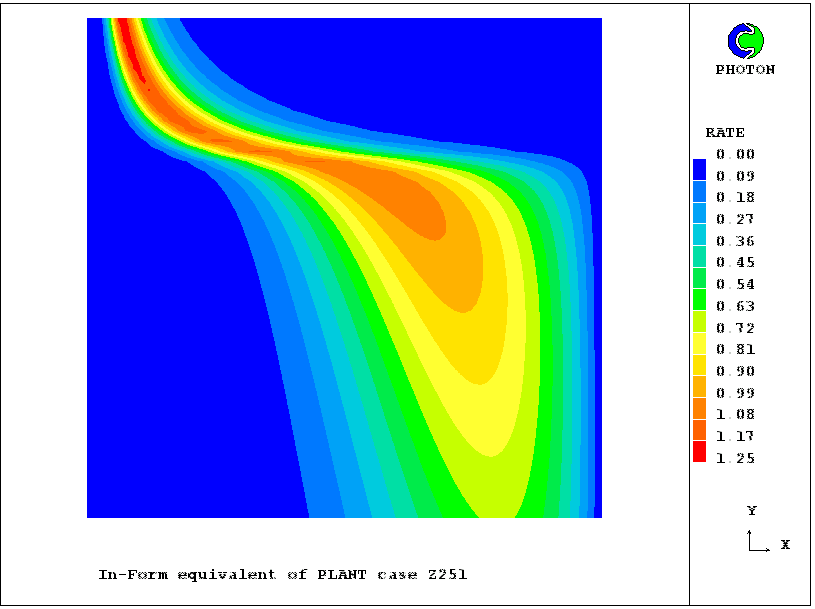
A single differential equation is being solved, namely that for the 'reactedness', RCTD; but a second variable, namely RATE, is computed for each location; it is the volumetric reaction rate.
It is the distribution of the latter with x and y which is displayed in this contour plot.
Case 492 illustrates the use of In-Form to simulate chemical reaction in a turbulent gas by way of the 'eddy-break-up' formula.
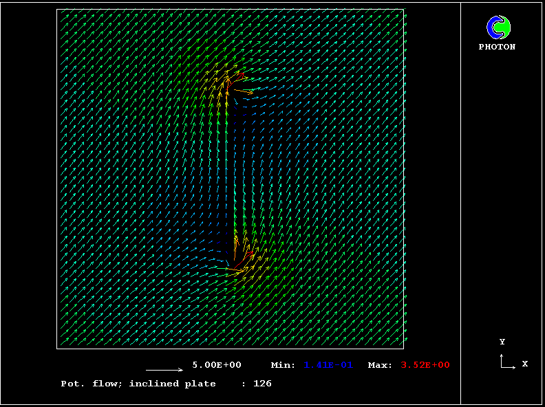
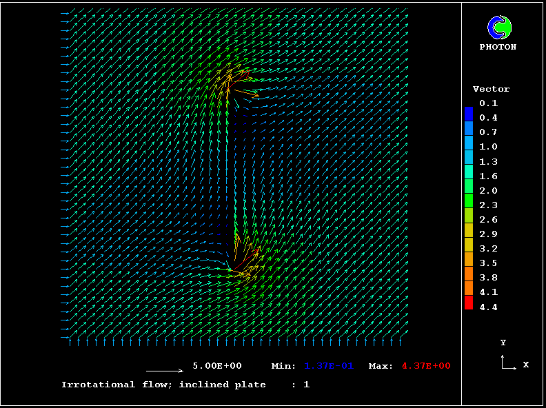
In-Form is used for setting the velocity potential, in the former, and the stream function, in the latter, at the boundaries of a domain in which a plate is held at an angle to the stream in which it is immersed.
The computed velocity vectors for the two cases are shown on-line here and here.
(SOURCE of VAR_NAME at VR_OBJECT_NAME is FORMULA)
The VR_OBJECT_NAME, like a patch name, marks the part of the domain inside which the source is to be applied; but it does so in geometry-related terms by way of lines in the Q1 file starting with >OBJ.
The object-describing lines usually appear below the source-describing lines in the Q1 file; but this is not necessary.
> OBJ, INFSRC_VARNAME, FORMULA
If the length of a line exceeds 68 symbols then the formula continuation is recorded in the next line, as follows:
> OBJ, INFSRC_VARNAME, FORMULA_BEGINNING$
> OBJ, INFSRC_VARNAME, FORMULA_CONTINUATION
[ (SOURCE , it should be mentioned, is not the only In-Form keyword which can be treated by this second method. Thus INFINI_, INFSTO_, INFST1 and INFMAK_ have the same effects as the In-Form statements starting: (INITIAL , (STORED , (STORE1 and (MAKE .]
The In-Form object-defining lines may be written to the Q1 file by way of any word-processor.
Also the In-Form object-defining expressions can be located in '.DAT' or '.POB' files. In this case SATELLITE reads them from these files and places them appropriately in the Q1 file.
Examples of both methods will now be described.
However that use is de-activated in favour of Method 2, as is shown here.
The two methods produce precisely the same solutions, with the trivial difference that that the SPEDATs echoed into Group 19 of the RESULT file appear in slightly different orders.
Case v147 exemplifies the use of Method 1 and Method 2 to set heat sources in an array of rods as described here.
Clearly, it is convenient to express all the sources for that object by means of formulae containing assignable quantities, namely the character variables VIN and MDOT.
The ability swiftly to implement new expressions for the reaction rate is especially valued by combustion scientists who are forever searching for ways to reduced the observed phenomena to order.
It is necessary to add at this point only that the syntax for attaching sources to such objects is similar to that for initial objects, as will now be illustrated.
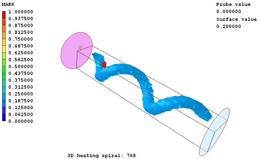
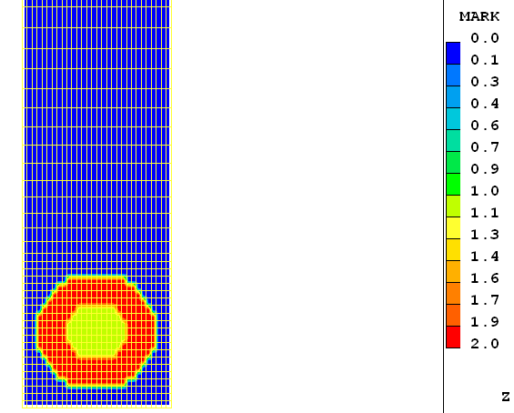
In order to create the required shape, which is shown here by displaying the surface of the marker-variable, MARK, the 'drilling technique' is employed.
That is to say that a sphere of constant radius is moved along a spiral trajectory in order to mark the cells through which it passes. The set of marked cells comprises the In-Form object.
A single-coil spiral can be formed from a ring by cutting it and moving the severed ends in an axial direction. In this case a two-loop spiral is required.
SPHERE(10+0.5*sin(xg),1.0+0.5*cos(xg), 1.0 , 0.2 )
Here:
where 1.0 is the Z co-ordinate of the start point of the spiral.
The Z co-ordinate of the final point of the spiral will be
1+0.5*XULAST=1+0.5*6.28=4.13
The complete In-Form statement will thus be:
(INFOB at PATCH1 is SPHERE(1.0+0.5*sin(xg),1.0+0.5*cos(xg),1.0+0.5*xg,0.2) with INFOB_1)
In order that they should be connected without a break, the Z co-ordinate of the starting point of the second coil should be equal to the Z co-ordinate of the final point of the first coil. Thus the Z co-ordinate should be calculated by the next formula:
4.14+0.5*xg
(INFOB at PATCH1 is SPHERE(1.0+0.5*sin(xg),1.0+0.5*cos(xg),1.0+0.5*xg,0.2) with INFOB_1)
(INFOB at PATCH1 is SPHERE(1.0+0.5*sin(xg),1.0+0.5*cos(xg),4.14+0.5*xg,0.2) with INFOB_1)
Moreover they can be incorporated into one statement, namely:
(INFOB at PATCH1 is SPHERE(1.0+0.5*sin(xg),1.0+.5*cos(xg),1.0+0.5*xg,$
0.2)+SPHERE(1.0+0.5*sin(xg),1.0+0.5*cos(xg),4.14+0.5*xg,0.2) with INFOB_1)
This would still be true if the formulae in the second statement had been different from those in the first, describing a straight cylinder rather than a continuation of the coil.
In library case 768, a constant source of 2.0 kilowatts is provided, thus:
(SOURCE of TEM1 at PATCH1 is 2000. with INFOB_1)
However, any formula recognised by In-Form could be provided.
It should be noted that 'at PATCH1' appears, not 'at INFOB_1'. In effect the In-Form object is acting as a qualifier, indicating into which cells of PATCH1 the source is to be provided.
This observation answers any question about the type of the source; for the type is dictated by the second argument of the the PATCH specification, which, in library case 768 is CELL.
This information immediately raises a further question, namely how many cells does the 'drilling' sphere actually mark?
One way of finding out would be to use the In-Form SUM feature to compute the total amount of the MARK quantity in the patch; but no exemplification of this idea yet exists.
However a solution to a similar problem will be discussed below in connection with the mass-flow sources of library case 785. If that example were followed in the present case, the actions could be:
Click here to see the MARK contours, which clearly show the geometry of the inlets and their relation the the grid.
Because In-Form objects know nothing of 'partially-blocked' cells, and regard each cell which they touch as wholly inside or wholly outside them, the edges of the inner and outer radii of the annulus are of course not truly circular.
The lines in the q1 file which create the two necessary In-Form objects can be seen by clicking here.
The following remarks can be made:
(INFOB at PATCH1 is SPHERE(0,:YIC:,:ZIC:,:RAD2:)-SPHERE($
0,:YIC:,:ZIC:,:RAD1:) with INFOB_2)
(SOURCE of U1 at PATCH1 is -1000.*VABS*VOL*U1 with INFOB_1)
(SOURCE of V1 at PATCH1 is -1000.*VABS*VOL*V1 with INFOB_1)
(SOURCE of W1 at PATCH1 is -1000.*VABS*VOL*W1 with INFOB_1)
where VABS is the square root of symmetrically-computed velocity-squared.
These are rather unsophisticated expressions which anyone who was seriously concerned about realistic simulations would certainly wish to alter.
However, as illustrations of the syntax of the source statement for In-Form objects, they suffice.
The formula following 'is' and the conditions after 'with; can be as complex as one wishes.
It suffices to look at only one set of the relevant source-related statements in the Q1 file, namely:
*** Secondary inlet V1 swirl flux
CHAR(FORM)
FORM=:USWIRL:*(ZG-:ZIC:)/SQRT((YV-:YIC:)^2+(ZG-:ZIC:)^2)
(SOURCE of V1 at INLET2 is :RHO1:*:USEC:/SECNF*:FORM: with INFOB_2)
about which the following explanatory remarks are appropriate:
Sources for sub-grid objects can be set in the same way as for other In-Form objects, thus:
(SOURCE of Var_Name at Patch_Name is Formula with Infob_N!Flags)
where
Infob_N is a special flag linking this source with the In-Form sub-grid object havng the current number N .
The 'type' of Patch (i.e. the second argument of the PATCH command) affects the magnitude of the source; thus, if the type is volume, then the source is multiplied by the SGO volume.
The flow resistance at point or line object with 1 number can be set by the following In-Form statement
PATCH(SGO,VOLUME,1,NX,1,NY,1,NZ,1,1)
(SOURCE of U1 at SGO is -1.*VABS*U1 with INFOB_1!line)
where the friction coefficient depends upon the square root of the symmetrically-computed velocity-squared quantity which is stored as VABS variable. The line flag (invoking LINEarization, and having nothing to do with the LINE SGO)is used for improvement of convergence. The size of '1.' constant is defined by the user.
The heat source equal 1.e6 W/m^3 per unit line or point sgo volume is set by next statement
PATCH(SGO,VOLUME,1,NX,1,NY,1,NZ,1,1)
(SOURCE of TEM1 at SGO is 1.E6 with INFOB_1)
If the heat source is set per unit line sgo length and equal 1.e3 W/m then the source formula should be 1.E3*LSGLN/LSGTL/VLFRIO/VOL where LSGTL is total length of lsgo and LSGLN is the length of the part of lsgo located inside one cell
PATCH(LSGO,VOLUME,1,NX,1,NY,1,NZ,1,1)
(SOURCE of TEM1 at LSGO is 1.E3*LSGLN/LSGTL/VLFRIO/VOL with INFOB_1)
PATCH(IN2,WEST,1,1,1,NY,2,2,1,1)
COVAL(IN2,H1,ONLYMS,HINL)
where HINL is inlet value of enthalpy.
Equivalent of this in 746 case is defined as follows:
(SOURCE of H1 at IN2 is coval(onlyms,HINL))
(SOURCE of H1 at INL2 is coval(ONLYMS,TWALLMAX*2))
FORM=pwl3(xg,0,0,.4*xulast,-.5*:twallmax:,.5*xulast,2.0*:twallmax:,xulast,:twallmax:)
PATCH(SW2,SWALL,1,NX,1,1,2,2,1,1)
(SOURCE of H1 at SW2 is coval(1.,:FORM:))
PATCH(IN2,WEST,1,1,1,NY,2,2,1,1)
(SOURCE of P1 at IN2 is coval(fixflu,rho1*UINL))
COVAL(IN2,P1,FIXFLU,RHO1*UINL)
Evidently, the commands are very similar.
(SOURCE of P1 at INL2 is coval(fixflu,RHO1*VELMAX*(1.-(2.*YG/YVLAST-1)^2)))
PATCH(OUT2,EAST,NX,NX,1,NY,2,2,1,1)
(SOURCE of P1 at OUT2 is coval(PCOF,POUT))
where POUT is outlet pressure value and PCOF is outlet pressure coefficient.
In this case 746 they are constants. But they can be described by formula. Also FIXP and FIXVAL can be used for PCOF.
(SOURCE of P1 at OUT2 is coval(PCOF*(YG/YVLAST)^2,POUT))
If the complete formula of a source is
PCOF*(YG/YVLAST)^2*(POUT-P1)
it can be converted easily to the standard C*(V-Phi) format be setting:
C=PCOF*(YG/YVLAST)^2
and
V=POUT.
PATCH(IN2,WEST,1,1,1,NY,2,2,1,1)
(SOURCE of U1 at IN2 is coval(onlyms,UINL))
COVAL(IN2,U1,ONLYMS,UINL)
(SOURCE of U1 at INL2 is coval(ONLYMS,VELMAX*(1.-(2.*YG/YVLAST-1)^2)))
PATCH(SW2,SWALL,1,NX,1,1,2,2,1,1)
(SOURCE of U1 at SW2 is coval(1.,UWMAX*XG/XULAST))