Encyclopaedia Index
MULTI-BLOCK GRIDS AND FINE-GRID EMBEDDING
(by I.Poliakov and V.Semin)
Contents:
- Introduction to CCM/MBFGE.
- Mathematical Background of CCM/MBFGE method.
2.1 Organization of the computational space.
2.2 Description of the LINK scheme.
2.3 MBFGE equations.
2.4 Unstructured Linear equation solver.
2.5 New Collocated (CCM-) method for CFD-problems.
2.6 Alternative discretisation Schemes for convection.
- Activation and use of MBFGE/CCM method.
3.1 MBFGE/CCM library.
3.2 Grid generation.
3.3 MBFGE/CCM activation.
3.4 Activation of physical models and built-in source terms.
3.5 Initial and boundary conditions.
3.6 Use of alternative convection schemes.
3.7 Activation and use of special options:
3.7.1 Swirling flow simulation.
3.7.2 Sliding grid simulation.
3.7.3 Darcy flows.
3.7.4 Shallow flow models.
3.8 GROUND influence on CCM/MBFGE calculations.
3.9 Use of IPSA with MBFGE/CCM.
3.10 Use of self-adjustment of relaxation parameter.
3.11 Automatic provision of friction at solid/liquid interface.
- CCM-switch in SATELLITE.
4.1 New options of READCO and MBFLINK commands.
4.2 How to convert existing Q1 or just created by SATELLITE menu to the Q1
for CCM method.
- Use of PHOTON to visualize results of the MBFGE calculations.
- References
1. Introduction to CCM & MBFGE.
CCM and MBFGE are alternative solvers of Navier-Stokes equations, which are available
as options in PHOENICS.
CCM stands for Collocated Covariant Method. Essentially CCM is a segregated
Navier-Stokes equation solver based on the collocated-velocity arrangement, with covariant
velocity projections, i.e. those aligned with the co-ordinate directions of the grid, as dependent variables. The solution of the equations is achieved by a
global algorithm, which employs SIMPLE-like procedure [1] with Rhie-Chow-like
interpolation [8]. As linear-equation solver CCM uses either LU-, or 2-step Jacobi
pre-conditioned conjugate-residuals solver [3].
MBFGE stands for Multi-Blocking and Fine Grids Embedding. The MBFGE solver is based on
the non-overlapping domain-decomposition method and provides the use of multi-block grids
(MBFGE grids) in CFD simulations with PHOENICS. The MBFGE grid for a problem comprises a set of separate grids, linked together through common boundaries. Separate grids in a MBFGE grid can be:
- grids created for distinct sub-domains of a larger total domain;
- finer grids embedded within coarser ones, or
- combinations of both.
The MBFGE link-scheme has the following main features:
- The cellls of sub--domain grids may adjoin in either a 'one-to-one' or 'one- to-many' manner, thus:
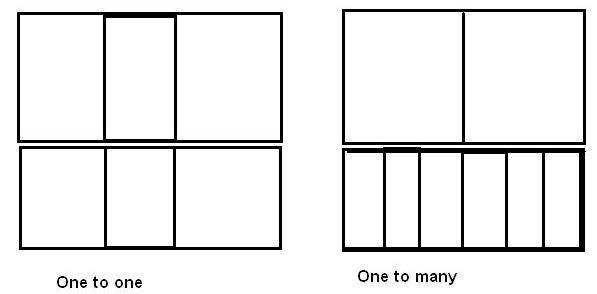
with however only integral ratios which are the same for all cells in the pair of adjoining sub-domains.
- There are no restrictions on the position of each sub-domain in the total domain, except that the cell-surface pair which adjoin must be north and south, east and west or high and low.
- Grids within each of the separate of separate blocks are structured, however the total grid can be regardes as unstructured, in that NX, NY and NZ can be forfferent for each.
- For solving the linear equations, the MBFGE method employs an unstructured version of LU- or 2-step
Jacobi preconditioned conjugate residuals solver. As a result the speed of convergence is
governed only by the overall number of cells and it is not affected by the number of
linked domains or links set in the MBFGE grid.
- For hydrodynamics problems, MBFGE uses the CCM algorithm.
- The link treatment in CCM for MBFGE is
developed in such a way, that it does not affect the global convergence, which is governed by exactly the same factors as for the one-domain CCM
simulation , namely:
- the character of a problem,
- overall number of computational cells,
- etc.), but
- not the number of linked cells northe type of set links (one- to-one or
one-to-many)
.
2. Mathematical Background of CCM/MBFGE method.
2.1 Organization of the computational space.
The CCM method is based on structured computational grids. It can employ all types of
grids available in PHOENICS, namely:
- cartesian
- cylindrical polar, and
- curvilinear (or BFC).
The organization of the computational space (i.e. the notation of axes; the index
notation; etc.) is described under appropriate entries to PHOENICS encyclopedia, as well
as in manuals (TR100 and TR200). The contents of this paragraph impliy that reader is
well familiar with the organization of PHOENICS computational space.
The MBFGE method is based on the domain-decomposition approach to facilitate the grid
generation for application problems with a complex geometry. Essentially, user should
subdivide the whole region into a set of rather simple domains, within each of which a
separate computational grid is generated. The union of all domains (or grids) covers the
whole region. In MBFGE method subdomains are to be put together without overlapping; i.e.
linked domains have only boundary surface (or surfaces) in common.
DOMAIN 1
Common DOMAIN 2
boundary
Common ^
boundary > DOMAIN 3
The domain decomposition approach gives the following advantages and new features to
PHOENICS simulations:
- The grid for any of the subdomains can be generated in a simple, straight-forward manner
using any available grid generator with PHOENICS interface.
- The solution regions requiring grid refinement can be isolated in separate subdomains by
embedding fine grid or a succession of fine grids.
- User may create library of geometrical objects/grids which can be put together or added
to some existing complex grid without necessity to rebuild the whole computational grid.
- In the future it provides rather covenient and natural way for splitting a problem into
smaller portions for parallel computation.
In MBFGE method, all grids created for subdomains (local grids) are structured - cells
are topologically cartesian brick elements. All kinds of grids available in PHOENICS can
be employed as local grids. Local grids are combined together to create global grid (or
global computational space). The MBFGE global computational space is topologically
unstructured, i.e. a neighbour in grid index space (say, cell J+1) may by far apart in
physical space.
At present, the MBFGE method uses the (X,Y,Z) notation along with (I,J,K) notation to
describe global computational space. It means, that all MBFGE grids are built as BFC grid
in PHOENICS notation, despite the actual topology of constituent grids.
The process of combining of local grids into global grid is called
below as stacking. MBFGE stacking employs layers of dummy cells to
separate local grids put into
the global one (see picture).
Later dummy cells are blocked
DOMAIN 1 DOMAIN n to prevent their use in the
computation. At present it is
j+1 achieved by setting the volume
j
< porosity (VPOR) to zero. For user it means that VPOR should DOMAIN 2 DOMAIN m be stored if MBFGE method is used (i.e. Q1 should comprise Dummy PIL command STORE(VPOR)). k k+1 < layers
For the problems without convection (for example, heat transfer problems) MBFGE method
enables to use arbitrary stacking of grids. However, for the CFD problems, MBFGE method
permits only the stacking, which provides uniform directions of all local system of
coordinates. It means that all local grids must have the same position of not only
(X,Y,Z)-, but (I,J,K)-coordinates.
It is also necessary to distinguish MBFGE stacking described above and that currently
provided by SATELLITE. The SATELLITE stacking is only a variant of these permited by MBFGE
and is as follows:
- By default, SATELLITE stacks domains linearly along the Z-axis. If 2D problem is set in
X-Y plane, then the satcking direction is X-axis.
- It is possible to change the stacking direction on any other present in the problem (see
p.2.2). However, the stacking will still be linear.
User is free to develop either add-on to SATELLITE, or his own grid generator which
will provide more compact stacking than that available in SATELLITE ver. 2.
2.2 Description of the LINK scheme.
The MBFGE link scheme consists of the following elements:
- The adopted stacking method described in the previous paragraph.
- The way to define and process connection between domains, or actually between cells,
faces of which form the common boundary.
- And the way to provide the MBFGE solver with that information.
By default, any (I,J,K)-cell in a structured grid is linked to the six immediate
neighbours: (I-1,J,K), ..., (I,J,K+1). In other words it has six links, one on each of six
faces. (It is not the case for cells at domain boundaries, but in that case missing links
are substituted by boundary conditions.)
In the MBFGE grid, a cell might have on one (or more) of its faces not only the links
mentioned above, but the link to a face of some (L,M,N) cell, or to faces of a group of
cells. These cells may be positioned in any place of global computational space. Below
only that kind of links as referred to as the MBFGE link or just link.
An Bn
Dom A Dom B
J Ae Bw J
I I
As Bs
Two types of links are distinguished in the MBFGE link-scheme:
- NATURAL links, are the links which preserve the same orientation of local (I,J,K)
systems. For example, link of the EAST-face of domain A (Ae) to WEST-face of domain B
(Bw), or link of the NORTH-face of domain A (An) to SOUTH-face of domain B (Bn) are
natural.
- NON-NATURAL links are the links of other kind. For example, link of the Ae-face to
Bn-face, or link of the Bs-face to As-face are non-natural links.
At present, only natural links can be used for simulation of CFD problems with MBFGE
method. Non-natural links may only be used for scalar problems without convection, for
example, heat-conduction, potential flows, etc. .
The MBFGE link-scheme is based on the non-overlapping approach. It means, that a cell
at the linked boundary of a domain can be linked only either to one cell (link
'one-to-one'), or to the whole number of cells from the other domain (link 'one-to-many').
There is no limit on the number of cells connected to one cell; it could be 1-to-5,
1-to-17, etc.. However, the type of connections should be uniform across the linked
surfaces of domains.
The linked surfaces in the MBFGE method are defined by special PIL command MBLINK (see
p.2.2). Actually, this command generates pair of LINK patches (one for
each linked domains) which spans define the size of common surfaces of linked domains.
Link patches are processed by MBFGE solver to fill special arrays which provide
information on the presence of links for a cell and, if some cell face has a link, the
adresses of first and last cells linked to it. User can get these information using
functions and subroutines described in p. 2.8.
As it was already mentioned, the type of cell-to-cell connection has to be uniform
across the link patch. If it is desirable for a user to introduced mixed connections
across the same common surface, it can be done, at present, only by setting several link
patches.
2.3 MBFGE equations.
In general, MBFGE solver treats the conservation equations in exactly the same way as
PHOENICS solver (see [6]), i.e. the finite- difference approximation of
balance equations is transformed into finite-volume equations of the form
Ap Fp = An Fn + As Fs + Ae Fe + Aw Fw + Ah Fh + Al Fl + At Ft + S
where Fi's are values of a solved variable in neighboring cells; Ai's are coefficients
and S is appropriate source term. The form of Ai's is exactly the same as in PHOENICS:
          Dens*Vel*Area       Exch_Co*Area/Dist     Dens*Vol/Dt
           ^Convection           ^Diffusion         ^Transience
Moreover, the values of coefficients for non-linked cell faces are calculated by the
same subroutines as for PHOENICS solver. They stored in the same arrays and can be
accessed by standard methods.
If a cell P (I,J,K) has a link at, say, SOUTH-face to some other cell (L,M,N), the
coefficient As is recalculated by MBFGE solver taking into account the actual inter-cell
connection. If the link is not one-to-one, but one to a number of cells, the term A*F
takes the form of Ai*Fi, where the summation covers all cells linked to the face. The sum
and Ai's values are calculated by MBFGE solver by balancing the fluxes passing through the
linked faces.
Due to the fact, that position of linked cell or cells in the global computational
space could be arbitrary, all variables in MBFGE method are solved for in the whole-field
manner.
On orthogonal grids source term for scalar variables is the same as produced by
PHOENICS solver after processing source patches. For collocated velocity projections it
comprises additional source terms which are calculated by MBFGE solver. These are the
pressure gradient and terms associated with the curvilinearity treatment.
On nonorthogonal grids MBFGE solver recalculates Ai's, as well as adds appropriate
terms to the source term.
As for PHOENICS solver, the balance equation is cast into the correction form before
the solution.
2.4 Unstructured Linear equation solver.
Finite-volume-equations, written for each cell in the global computational space, form
a set of simultaneous algebraic equations. For one domain problems a matrix of that system
has some regular structure (usually it has only a number of non-zero diagonals). This is
not the case for a general multi-block problem.
A variety of iterative methods is available to solve systems of linear algebraic
equations arising for one domain problems (SOR, Stone, MSIP, etc.). Most of them are based
on the use of the existent regular structure of the system matrix, thus these methods can
not be applied directly to solve the sytem of linear equations for a general MBFGE case.
The problem could be tackled by the introduction of additional iterative processes to
treat the wrongly positioned elements explicitly. However, this procedure may
significantly reduce the global convergence speed.
The alternative way to solve the system of linear equations for a multi-domain problem
consists in the use of a special solver, which is able to treat linear equations sytems
with unstructured matrices immediately. The MBFGE method employs that kind of a solver.
The unstructured linear equations solver is developed on the basis of preconditioned
conjugate residuals algorithm [3].
By default, the LU-preconditioning is used. User can change it on the 2-step Jacobi
preconditioning by setting LSG5=T. The LU- peconditioning usually provides faster
convergence, than 2-step Jacobi, however it requires more additional memory. For this
reason 2-step Jacobi preconditioning can be recommended when there is lack of computer
memory available.
2.5 New Collocated (CCM-) method for CFD-problems.
For the CFD problems MBFGE solver employs CCM solver. CCM is a segregated Navier-Stokes
equation solver based on the collocated grid arrangement and covariant velocity
projections as dependent variables. The coupling of equations is achieved by a global
iteration algorithm, which employs SIMPLE-like procedure [1] and Rhie-Chow-like
interpolation [8].
This entails that cell-centered velocity projections Uc, Vc and Wc are solved-for variables. They are aligned with the grid lines. The grid-line direction in the center
of a cell is defined by line connecting the centers of appropriate opposite faces. In
CCM/MBFGE notation, the first-phase velocities are UC1, VC1 and WC1, thus Q1 should
comprise SOLVE(UC1,VC1,WC1) command.
The face-centered velocity projections have exactly the same meaning, as in the staggered
PHOENICS solver; they are convection-flux velocities. However, in CCM they are not solved
for, but calculated using Rhie-Chow like interpolation procedure. The face-centered
velocity projections are stored in U1, V1 and W1 respectively.
Cartesian velocity components UCRT, VCRT and WCRT calculated for curvilinear grids are
attributed to the cell-centers.
2.6 Alternative discretisation Schemes for convection.
The general transport equations solved by PHOENICS includes transient, convection,
diffusion and source terms. To derive finite volume equations, certain numerical schemes
are used for discretisation of these terms (see [6] or appropriate
entries in POLIS). By default, the numerical schemes used in MBFGE/CCM for the
approximation of the diffusion and convection contributions are exactly the same as in
standard staggered PHOENICS solver.
Thus the diffusion-convection interaction is accounted for by the
"hybrid-interpolation" scheme (see DIFCUT entry to PHENC, or [6]), which resolves into the classical upwind differencing scheme (UDS-
scheme) for convection dominant flows.
The UDS scheme is very robust; but in the CFD simulation of the convection-dominated
physical problems it usually suffers from the severe numerical diffusion, which can
prevent from receiving the accurate solution, especially for the problems with rather
strong gradients of variables. The collocated MBFGE/CCM solver includes a set of
optional alternative convection schemes to alleviate the influence of the numerical
diffusion by introducing the treatment of the convection terms with a high accuracy. The
schemes available at present are briefly described below.
The straightforward approach to increase the approximation order of the UDS-scheme (for
example, to second order in SOU-scheme [10], or third order in QUICK-scheme [11]) resulted
in algorithms which tend to give rise to random oscillations of the solution in the
regions of strong gradients. This fact is in the agreement with the conclusion of the
Godunov's (1959) theorem [12] concerning the inevitable production of oscillations by
linear convective scheme of accuracy higher than first order. The MBFGE/CCM solver
includes as an option QUICK-scheme.
In recent years, a set of the non-linear algorithms has been proposed by various
authors to suppress the parasitic oscillations. All these methods are based on the
analysis of the local solution behavior and can be described as a sequel to the Godunov's
first- order Lagrangean scheme [12].
The first robust monotonic second-order convective scheme was the monotonic piecewise
linear scheme (MINMOD-scheme) of Van Leer [13], where the slab averaging of the solved
variable is used instead of mesh point values as in Gogunov's scheme and monotonicity is
enforced by suitably adjusting the second-order terms. Better results in resolving the
sharp gradient regions were achieved by the monotonic second-order upwind algorithm
(SUPER-BB-scheme) of Roe [14], which has been originally developed for the prediction of
the inviscid compressible flows. Both schemes belong to the class of TVD-schemes (TVD
stands for Total Variation Diminishing) and are included into the CCM/MBFGE convection
schemes' set.
Among the recently proposed procedures to express and develop TVD- schemes it is worth
mentioning the notion of NVD (Normalized Variable Diagrams) of Leonard [15]. The
NVD-representation can significantly simplify the test on whether some convective scheme
is TVD or not. Using the NVD-technique Leonard developed the new SHARP-scheme (Simple
High-Accuracy Resolution Program), which is a monotonic version of his QUICK-scheme.
Similar to SHARP is the simpler SMART-scheme of Gaskell and Lau [16], which is based on
piecewise characteristics. The MBFGE/CCM solver includes as an option SMART-scheme.
The alternative convection schemes are implemented in the CCM/MBFGE solver using the
deferred correction method. It means that all the additional terms, arising in the general
transport equation after it is discretized using some higher order convection scheme
instead of default UDS-scheme, are calculated on the solution from the previous iteration
and added to the source term.
All the convection schemes available in the CCM/MBFGE solver (i.e. QUICK, MINMOD,
SUPER-BB and SMART schemes) can be applied to any solved variable (including collocated
velocities), provided that the convective term is active for it. Details of their
activation can be found in p. 2.6.
3. Activation and use of MBFGE/CCM method.
3.1 MBFGE/CCM library.
To help and simplify the familiarisation with and learning of the CCM/MBFGE method,
SATELLITE library includes CCM/MBFGE library. This library can be accessed either through
submenu 'Library' of SATELLITE menu, or by typing SEELIB(F) on the SATELLITE command mode
prompt. The library file resides in D_SATELL/D_OPT/D_MBFGE subdirectory of main PHOENICS
directory.
Cases included into CCM/MBFGE library can be loaded either through submenu 'Library'
of SATELLITE menu, or by entering LOAD(Fnnn), where 'nnn' is the case number, on the
SATELLITE command mode prompt.
The CCM/MBFGE library consists of two parts: CCM library and MBFGE library. First part
includes cases set on one domain grids to run with CCM solver. Most of the cases included
in it are set to be simulated either with CCM solver, or PHOENICS staggered solver (to
chose the latter, user should set PIL variable LCCM defined in Q1 to FALSE). The
MBFGE-library includes cases set on multiblock grids (including grids with fine grid/grids
embedding). These cases can be run with MBFGE solver. It is recommended to the user to
study them not only as examples of MBFGE solver activation, but as the examples of the
MBFGE grid generation.
Along with cases set for some CFD problems, the CCM/MBFGE library includes the case
(case F150), which is essentially the set of PIL commands to activate solution for
collocated covariant velocity projections (or CCM/MBFGE methods). This case can be loaded
in Q1 by the following PIL commands:
NOWIPE= T
LOAD(F150)
It is recommended to load it after the grid generation part of a Q1, but before
settings of boundary conditions. Examples of its use can be found in the most of CCM/MBFGE
library cases.
3.2 Grid generation.
Both CCM and staggered PHOENICS solvers are based on structured computational grids.
They can employ grids of three distinct kinds, namely:
- cartesian
- cylindrical polar, and
- curvilinear (or BFC).
The details of the grid specification, as well as grid generation using SATELLITE can
be found under appropriate entries of PHOENICS manuals (TR100, TR200 and TR219) and
encyclopedia. In addition to SATELLITE, user may also employ any other available to him
grid generator to build BFC grids. That alternative grid generator must be able to create
grid file in XYZ-format.
MBFGE solver is based on the computational grids which are built as a union of
structured grids created for each of the blocks using the standard grid generation
technique. Grids are connected through common surfaces. At present, overlapping is not
permitted. Cells' faces at the interface can be connected either one-to-one, or one-
-to-many ('many' must be whole number of cells).
NOTE !, that at the surfaces defined as a LINK (details see below) all cells has to be
connected in the same way, i.e. either one-to -one, or one-to-two, or one-to-three, etc..
If it is desirable to have regions with different connections along the same common
surface, user should introduce several LINKs instead of one.
Note the difference between PHOENICS specification of cartesian or cylindrical polar
grids and that of curvilinear grids, which is important for MBFGE method. The first two
kinds of grids are defined using fraction arrays; there is no special arrays to store
coordinate of cells' vertices (X,Y,Z arrays). On the contrary, BFC grids are defined using
X, Y, Z -arrays, which provides the way to store grid information for all domains of
multiblock grid. Thus:
- All the multiblock grids (or MBFGE grids) are defined as the BFC grids in PHOENICS, even
though the actual geometry of all blocks is cartesian or polar cylindrical.
At present, the generation of the MBFGE grid can be schematically represented as three
successive steps:
- grid generation for each of the subdomains;
- stacking of the separate grids into one computational grid; and
- definition/introduction of necessary links.
Let's consider these steps in details, implying that SATELLITE will be used for the
second and third steps. It is possible for the user to create and use alternative grid
generator and/or GROUND coding for SATELLITE, which will incorporate all steps. In the
latter case, it is desirable to obtain additional information, which is available from
CHAM development team.
The SATELLITE treats grids for the subdomains independently while stacking them into
one MBFGE grid, thus all subgrids have to be present in the working directory as separate
XYZ-files. XYZ-files should be named as
NAME1, NAME2, ..., NAMEn
where NAME (string of up to four letters) is common name for all subgrids of a
multiblock grid; n is the total number of blocks. The numbering order of subgrids is not
important.
All NAMEi files has to be created at the first step or copied from a library of
previously created grids. If SATELLITE grid generator is used to build subgrids the steps
are as follows:
- declare grid as the BFC-grid by setting BFC=T in Q1, or choosing that grid type from
PHOENICS menu;
- introduce necessary PIL-commands into Q1, or create geometry in the PHOENICS grid
generator menu;
- exit SATELLITE and rename produced XYZ file.
Note, that all subgrids can be created in the single Q1. It can be achieved by dumping
each created subgrid to disk by DUMPC(NAMEi) PIL-command. All MBFGE examples in the
CCM/MBFGE library had been created using that method.
In case of an alternative grid generator user should follow its instructions to create
subgrids and write them to disk in PHOENICS XYZ format.
Once all subgrids had been created, it is possible to proceed to the second step. As a
result of this step, SATELLITE will stack separate subgrids together and create single
MBFGE computational grid. It is achieved by the following PIL-commands:
BFC= T; NUMBLK= n; READCO(NAME+)
READCO() command will read in NUMBLK XYZ-files (with names NAME1, ..., NAMEn) and put
them them into single grid file using rules described in pp. 2.1 and 2.2.
By default subgrids are stacked by SATELLITE either along Z-axis, or along X-axis for
cases set in X-Y plane. It is possible to change the stacking direction by specifying the
new one in the argument of READCO:
READCO(NAME+X), or READCO(NAME+Y), or READCO(NAME+Z)
Note, that for 2D cases the alternative direction must be present.
The third step consists in the definition of necessary links, which is achieved by the
MBLINK commands. The formats of MBLINK command are as follows:
MBLINK(m,SOUTH,n,NORTH) or MBLINK(j,IN,k)
First command defines LINK between domain 'm' at its SOUTH-side and domain 'n' at its
NORTH-side; while the second defines domain 'j' as embedded into domain 'k'.
After processing READCO(NAME+) and MBLINK() commands, SATELLITE creates PATCHes with
MBD... and MBL... names accordingly (see pp. 2.1 and 2.2).
User can check positions of defined PATCHes by investigating contents of RESULT file after
the run of EAREXE (to initialize Q1 contents print-out into RESULT file user should put
ECHO=T in it). It can be recommended to check positions of LINK PATCHes introduced by
SATELLITE before proceeding to the setting and simulation of the problem itself.
To summarize the MBFGE grid generation consider possible scheme of Q1 which
incorporates three steps described above:
- Create local grids for all defined subdomains:
BFC= T;
GSET(D,NX1,NY1,NZ1,LX1,LY1,LZ1) ... GSET commands necessary to create grid for the 1st
somain.
DUMPC(MBGR1)
GSET(D,NX2,NY2,NZ2,LX2,LY2,LZ2) ... GSET commands necessary to create grid for the 2nd
somain.
DUMPC(MBGR2)
... And so on for all domains.
NOTE ! separate grids might be created using SATELLITE menu.
- Combine local grids into the single computational space:
NUMBLK = N; READCO(MBGR+)
- Set necessary links between subdomains:
MBLINK(2,IN,1); MBLINK(2,EAST,3,WEST); etc.
All examples of Q1 in MBFGE library are built according to that scheme.
3.3 MBFGE/CCM activation.
The PIL commands used for the CCM/MBFGE activation may be divided into four groups.
First group comprises settings, which has to be used to activate CCM/MBFGE solver and are
the same (with minor variations) for all MBFGE or CCM cases.
The second group includes setttings which are used to define grid geometry type.The
third group consists of switches to activate special techniques available in CCM/MBFGE
(high order convection schemes, the NX=1 simulation of swirling flows, etc.). The first
and second groups are described in this paragraph. The third type settings are detailed in
pp. 3.6 and 3.7.
All other PIL-commands which are usually used in Q1 and are not specific to CCM/MBFGE
(for example, initialization of variables, activation of various physical models, etc.)
may be attributed to the fourth group. Their description can be found under appropriate
entries of PHENC. Some notes on their use for MBFGE can be found in pp. 3.4 and 3.5.
PIL commands to activate CCM/MBFGE solver are as follows:
- Settings common for CCM and MBFGE:
- CSG3=LCRU. This line activates CCM/MBFGE solver; the problems is simulated by CCM/MBFGE
algorithm using LU-preconditioned conjugate residuals solver as linear equation solver.
The latter might be substituted by 2-step Jacobi preconditioned one if LSG5=T.
- Activate, if necessary, solution for collocated velocities: SOLVE(UC1,VC1,WC1) Activate
whole-field solution for all solved variables: for example SOLUTN(P1,Y,Y,Y,P,P,P); etc.
- Additional setting for MBFGE:
- Store volume porosity: STORE(VPOR).
PIL commands to specify the kind of geometry for CCM/MBFGE solver are as follows:
- For the CCM solver (or one domain simulation), all standard PIL- variables are valid to
specify the type of orthogonal geometry:
CARTES=T cartesian grid;
CARTES=F polar cylindrical grid;
BFC=T orthogonal curvilinear grid.
- By default, all MBFGE grids are treated as cartesian, despite the fact that BFC=T. There
is special variable to specify the grid as curvilinear, thus switch on the appropriate
treatment:
LSG3=T orthogonal curvilinear grid.
- The treatment of nonorthogonal grids in CCM/MBFGE solvers is different from that in
PHOENICS. To activate this treatment user should use the following commands:
NONORT=F;
LSG3=T; LSG4=T
NOTE, LSG3=T settings is necessary only if convection is present in the case. For the
case with diffusion only LSG4=T is enough.
3.4 Activation of physical models and built-in source terms.
Most of physical models, built-in or GREX-coded sources for scalar variables and models
to introduce thermo-physical properties of media available for PHOENICS solver are also
available for CCM/ MBFGE solver. User should refer to the approprite encyclopedia entry to
find the description of PIL commands necessary to activate the model under question. The
list of available models includes:
- Calculation of thermophysical properties of gases, fluids and solids through PROPS file
and GREX-subroutines.
- The built-in pressure source term in the enthalpy or temperature balance equation.
- Conjugate heat transfer model.
- All available in PHOENICS models of turbulence, except Reynolds stress-and-flux
transport model. NOTE !, necessary boundary condition should be set for the collocated
velocity projection instead of the stagerred ones.
- Coriolis forces for horizontal flows, which are activated by CORIOL parameter.
At present CHEMKIN, GENTRA, stresses in solids model and radiation model based on the
view-factors calculation are not available for use with CCM/MBFGE.
There are certain differences in the activation of the following physical models:
More details of the coriolis and centrifugal, as well as buoyancy forces activation can
be found in MBFGRN.FOR file, which resides in /phoenics/d_earth/d_opt/d_mbfge
subdirectory.
In general, if some physical model (available as part of PHOENICS installation or coded
by user for PHOENICS solver) is implemented as an algorithm user should consult CHAM
development team to check for its applicability to CCM/MBFGE.
There are the following rules for the models based on additional source terms to
PHOENICS equations, which can be used to check on whether or not some model in question
can be applied without modifications to CCM or MBFGE:
- Special consideration should be given to the velocity components or projections used (if
any) in the model.
- If model is based on calculations of derivatives of some stored variable, it needs
modification to provide proper treatment of linked boundaries. This modification can be
done using LINK subroutines described in p. 3.8.
3.5 Initial and boundary conditions.
In CCM/MBFGE solver initial and boundary conditions, as well as additional sources, are
introduced in exactly the same manner, as these for PHOENICS solver. Thus, user should
specify appropriate PATCHes and set COVAL() statements for solved variable. However, there
are certain differences described below:
- No-slip boundary conditions should be applied to all solved collocated velocity
projections (UC1, VC1 or WC1).
- To specify uniform initial flow field on curvilinear grids or set inlet at the
curvilinear surface (details can be found either in PHENC, or source file of GXBFC
subroutine) user should set GRND2 as VALue for P1, UC1, VC1 and WC1 instead of GRND1 for
PHOENICS solver.
For MBFGE grids user may use MPATCH() command instead of standard PATCH(). It has the
following format:
MPATCH(NB,NAME,TYPE,IXF,IXL,IYF,IYL,IZF,IZL,ITF,ITL)
Here NB is the number of the domain at which the patch NAME is set. Other arguments
have exactly the same meaning as for PATCH(). The difference is in the fact that
IXF,IXL,...,IZL should be specified as (IX,IY,IZ) local for NB-domain. SATELLITE will
process MPATCH and transform IXF,IXL,...,IZL into global (IX,IY,IZ) according to the
stacking used by it. NOTE, in the RESULT file all MPATCHes are printed out as standard
PATCHes with global (IX,IY,IZ).
3.6 Use of alternative convection schemes.
At present, the following high-order numerical schemes are included in CCM/MBFGE solver
as optional (instead of default UDS-scheme) for the approximation of convection terms:
- QUICK -scheme by Leonard [11];
- MINMOD -scheme by Van Leer [13];
- SUPER-BB-scheme by Roe [14];
- SMART -scheme by Gaskell and Lau [16].
Details of the mathematical formulation of these schemes can be found either in the
appropriate references, or in the entry SCHeMe of PHOENICS encyclopedia.
Current implementation has the following main features:
- Any alternative convection algorithm is applied to the whole computational domain, i.e.
up to domain boundaries.
- All the possible obstacles in the computational domain are treated automatically. It is
understood by the obstacle/blockage the settings of VPOR to 0; or PRPS to 'solid' value;
or the face porosities EPOR, NPOR, HPOR to 0.
- All patches related to the convection transport of the variable under consideration are
treated automatically.
To activate the alternative convection treatment in the MBFGE/CCM solver user should
set LSG7=T in Q1. Than it is necessary to provide the information on which scheme must be
applied to what solved variable. It should be done by introducing into Q1 the following
lines:
SCHMBEGIN
VARNAM VAR1 SCHEME MINMOD
VARNAM VAR2 SCHEME SUPERB
VARNAM VAR3 SCHEME SMART
VARNAM VAR4 SCHEME QUICK
SCHMEND
Here SCHMBEGIN and SCHMEND are keyword-brackets; VARNAM and SCHEME fixed keywords;
VAR1, ..., VAR4 are the names of solved variables, and MINMOD, SUPERB, SMART, or QUICK are
keywords to designate the appropriate numerical algorithm, which will be applied to the
variable, provided that convection term for it is active.
It is necessary to note the following:
- If the variable is solved, but its name is not included in that list, the convection
term for it is treated by the default UDS-scheme.
- High-order convection schemes can be applied as to all solved scalar variables (like KE,
EP, temperature, etc.), as well as to the collocated velocities UC1, VC1 or WC1.
- User can apply either the same scheme to all solved variable with active convection
terms, or use any mixture of schemes. For example UC1 and VC1 are treated by
SUPERB-scheme, while KE and EP by MINMOD-scheme.
- By default, alternative convection schemes are applied to the variable starting from the
first solution sweep. However, user can specify other sweep as a starting point by
assigning its number to the ISG1 variable in Q1.
User is advised to study various examples of schemes' activations and use, which can be
found in MBFGE/CCM library.
3.7 Activation and use of special options:
3.7.1 Swirling flow simulation.
The CCM/MBFGE module provides special option for the simulation of laminar or turbulent
swirling flows taking place in axisymmetric geometries.
The problem should be defined and set as 2D problem, using Z, as axis of symmetry, Y,
as radial direction and X, as circumferential direction (NX=1). Along with VC1 and WC1
velocity projections, which are normally solved for in the cases set in Y-Z plane, user
should activate solution for UC1. Set no-slip or other suitable boundary conditions for
UC1.
To activate treatment of UC1 as swirling velocity component user should specify in Q1
file LSG6= T. Other CCM/MBFGE variables (for example, LSG4 to activate the traetment of
nonorthogonality, etc.) should be set according to the problem under consideration.
Examples of cases set to simulate swirling flows using described option can be found in
CCM/MBFGE library: cases 105 and 110 for CCM; cases 208 and 215 for MBFGE.
NOTE !, that swirling flow problems can be simulated as 3D problem (NX>1), without
using LSG6 variable. However, if the flow is uniform in circumferential direction, the
speed of convergence is very low. For these reason 3D simulation of swirling flows can be
recommended only if there are flow variations in circumferential direction.
3.7.2 Sliding grid simulation.
The MBFGE method provides the special type of a link to simulate the flows which take
place in domains one part of which is moving in respect to the other. That type of flows
can be found, for example, in stirring reactors, turbines, etc..
The fact that one domain is moving in respect to the other is accounted for by the
SLIDING link and special patch, which covers the moving domain. Sliding link is introduced
by changing the standard part of the link patch, i.e. MBL, to MBS. For example, the
following link between domain M and N is sliding:
MPATCH(m,MBSm.n,NORTH,1,NXm,NYm,NYm,1,NZm,1,LSTEP)
MPATCH(n,MBSn.m,SOUTH,1,NXn, 1, 1,1,NZn,1,LSTEP)
At present, only one sliding link per multi-block grid is permitted by MBFGE solver.
Moreover, the sliding link has to be introduced between the NORTH face of one domain and
SOUTH face of the other domain. It means, for example, that the geometry of the
multi-block grid to represent the rotation of one domain in respect to the other should be
build using X as circumferential coordinate, Y as readial direction and Z as axis of
rotation (see MBFGE library cases 218, 219 and 220).
There two patches with fixed names 'SLIDRT' and 'SLIDMV' to mark the moving domain (see
cases 218, 219, 220 and 221):
MPATCH(n,SLIDRTn,CELL,1,NXn,1,NYn,1,NZn,1,LSTEP)
MPATCH(n,SLIDMVn,CELL,1,NXn,1,NYn,1,NZn,1,LSTEP)
Both patches should be set to cover the whole extent of the moving domain. Patch
'SLIDRT' marks domain as rotating domain. Values of angular velocity and position of the
axis of rotation are set through PIL variables ANGVEL, ROTAXA, ROTAYA, ROTAZA, ROTAXB,
ROTAYB and ROTAZB (see ROTA entry to PHENC and library cases). The angular velocity vector
is directed along Z axis; angular velocity is positive when rotation of cartesian X-axis
to Y-axis is counter clock-wise, as seen from the end of the vector.
Patch 'SLIDMV' marks domain as domain which moves along the surface of other domain
with transitional velocity U. Its value is passed to MBFGE solver through PIL variable
RSG2. Positive U value means that the domain is moving in the positive direction of
X-axis.
In transitional cases and rotational cases set for only a sector of axisymmetric
geometry user should introduce XCYCLE condition. It is achieved by using READCO(Y+)
command and choosing the same number of cells across the sliding link (see library cases).
3.7.3 Darcy flows.
Current release of CCM/MBFGE method includes special treatment to provide for Darcy
flows simulation. There is no special switch to turn it on. The treatment is automatically
activated once user set patches on UC1, VC1 or WC1 to introduce flow resistance.
Case 108 in CCM/MBFGE library gives an example of the Darcy flow simulation
3.7.4 Shallow flow models.
The CCM/MBFGE module provides two special models for the simulation of shallow flows.
The 3D flow can be defined as shallow, if its geometrical size in one dimension (or depth)
is much smaller than the sizes in two other dimensions. The water flows in rivers or sea
bays are examples of shallow flows. In general, that kind of flows can be simulated using
full 3D Navier-Stokes equations by CCM/MBFGE solver. However, the fact that the flow depth
is much smaller than the characteristic width and length, can be used to simplify the
Navier-Stokes equations and provide more robust algorithm.
NOTE !, that at present, the coordinate direction adopted as 'shallow' in CCM/ MBFGE
module is that along Z-axis. It means that only the cases set using Z to define flow depth
can be treated by CCM/MBFGE shallow flow option.
There are two logical parameters to activate shallow water models available in the
CCM/MBFGE module. The parameters and the models are described below:
- LSG8, when set to TRUE, activates the 2D shallow flow model for the solution of 3D
Navier-Stokes equations. The 2D shallow flow model consists in the following:
- The pressure-correction equation is solved in 2D form, which is deduced from the full 3D
equation by integrating along the Z-direction.
- Accordingly, the Wc velocity component is calculated by the integrating the continuity
equation.
- The momentum equations for Uc and Vc components are solved in the 3D form. However,
certain terms, which has Depth/Length order and thus they are negligible for the shallow
flows, are omitted.
- Transport equations for all other solved variables are solved in ordinary 3D form.
- LSG10, when set to TRUE, activates the 3D shallow flow model for the solution of 3D
Navier-Stokes equations. This model consists in the following:
- The momentum equations for Uc, Vc and Wc velocity components are solved in the truncated
form. The truncation is related to the terms, which has Depth/Length order of magnitude.
It should be noted that the form of Uc- and Vc-equations is exactly the same as mentioned
above for 2D shallow model.
- All the other equations, including the pressure-correction equation are solved in the
standard 3D form.
NOTE !, that 2D shallow flow model is implemented for CCM problems only (i.e. for one
domain simulations) and can not be used for multiblock grids. The 3D shallow flow model
(LSG10=T) can be used as for CCM, as for MBFGE cases.
Examples of the use of the 2D and 3D shallow flow models for a 3D flow simulation can
be found in the CCM/MBFGE library.
3.8 GROUND influence on CCM/MBFGE calculations.
The CCM/MBFGE module can be influenced by user in practically the same manner as all
others PHOENICS modules. Thus the presentation of this paragraph is based on the
presumption that the reader is well familiar with main rules of FORTRAN programming for
PHOENICS. If it is not the case, user should start reading from appropriate paragraphs of
PHOENICS lectures, manuals or encyclopedia entries.
Two kind of FORTRAN module are accessible to the user: the MAIN program of EARTH, and
GROUND/GREX subroutines. There are only two parameters in the MAIN program, which are
specific for dimensioning the arrays used in MBFGE module:
- NDM - set the maximum number of blocks in the MBFGE grid;
- NDMB - set the maximum number of links per block.
By default, NDM = 10 and NDMB = 6. The user may increase/decrease these values and
rebuild EARTH in the standard way.
All the ways to influence EARTH through FORTRAN coding introduced into GROUND/GREX
subroutines are also available to the user of CCM/ MBFGE method, i.e. user may modify
solved equations by adding new source terms or modifying coefficients; introduce necessary
thermo- dynamic properties of media; set complex boundary conditions; and etc. The general
rules of the use of GROUND groups; of retrieving/ placing information from/to F-array; and
of the work with PHOENICS arrays' indices are exactly the same as in standard EARTH.
However there are several remarks worth mentioning:
- Momentum equations solved in CCM/MBFGE module are formulated for collocated velocity
components UC1, VC1 and WC1. Accordingly, all the related modifications should be
introduced into equations solved for UC1,VC1, or WC1. Block location indices for
collocated velocities may be easily retrieved using LBNAME function (for example, IUC1=
LBNAME('UC1')).
- CCM method works on one domain grids; thus FORTRAN coding may be created in absolutely
the same manner as for standard PHOENICS solver.
- MBFGE method differs from CCM in the presence of linked cells. For a writer of GROUND
coding, it basically means that special attention should be paid to the way of getting
values from the neighboring cells. Accordingly, if user GROUND coding involves only
'in-cell' calculations, i.e. formulae to be coded do not include derivatives of variables,
then the FORTRAN coding can be created using the same technique as for standard PHOENICS.
For the GROUND coding, which involves 'inter-cell' calculations, the user should use a set
of special subroutines provided in MBFGE for links treatment. These subroutines are
described below.
- The organisation of the solution algorithm in CCM/MBFGE method differs from that in
staggered PHOENICS solver. For this reason, user should pay special care to the
modifications, which can affect it.
There is a set of special subroutines to provide the user with the tools for the
treatment of links in GROUND coding. It includes the following subroutines and functions:
| LDMN(IX,IY,IZ) |
- returns TRUE if (IX,IY,IZ)-cell belongs to one of the domains. It can be also used
for CCM, than it returns TRUE if 1<=IX=<NX, 1<="IY=<NY," and 1<=IZ=<NZ. |
| LLINK0(IJK) |
- returns TRUE if IJK-cell has at least one link. IJK is a whole-field index of
(IX,IY,IZ)-cell, i.e. IJK = IY + (IX-1)*NY + (IZ-1)*NX*NY. |
| LLINK(IDIR,IJK) |
- returns TRUE if IJK-cell has a link in the IDIR direction. IDIR has the same meaning
as for PHOENICS solver, namely IDIR=1 corresponds to NORTH-direction; 2 - SOUTH; 3 - EAST;
4 - WEST; 5 - HIGH; and 6 - LOW. |
| LINKD(IDIR,IJK,NF,NL) |
- returns the direction of the linked face for the cells (from NF to NL) linked to the
IDIR-face of a current IJK-cell. NOTE !, call to LINKD() must be preceded by the call to
GETFLI(), moreover the signs of NF, NL are important. |
| SSCLNK(IDIR,IJK,ISC0) |
- returns an average value of the scalar variable for the cells linked to the
IDIR-face of a current IJK-cell. Here ISC0 is absolute zero-location index of the
variable; for slab- wise arrays it is zero-location index of the first slab. Sign of
IJK defines type of the variable: if IJK>0 then ISC0-variable is slab-wise, else it is
whole-field. There are two types of averaging: if ISC0>0 then SSCLNK() returns volume
average; else it returns an arithmetic average. |
| GETFLI(IDIR,IJK,NF,NL) |
- returns first NF and last NL indices of cells linked to the IDIR-face of the current
IJK-cell (NF, NL, IJK are whole-field indices). NOTE !, that GETFLI() can be called only
if LLINK(IDIR,IJK) is true. NOTE !, that NF, NL could be negative for 'unnatural' links. |
| GETIJK(IJK,NX,NY,IX,IY,IZ) |
- returns IX, IY and IZ for a whole- field index IJK. NOTE !, IJK must be positive. |
There is also set of auxiliarily subroutines, which can be used in GROUND coding for
CCM/MBFGE module. These subroutines provide check for the presence of blocked cells in the
computational region and they can be subdivided into two groups: the subroutines to carry
out check for a current cell, and that to check neighboring cells.
Current cell is treated as blocked if the value of VPOR<=0 or value of PRPS>=SOLPRP. The cell neighboring to
the current cell is treated as blocked if it has either VPOR<=0, or PRPS>=SOLPRP, or if the value of
face-porosiry array in the appropriate direction is zero. All subroutines are pared; the
other subroutine in a pair does not check for PRPS value if the variable under
consideration is a temperature (TEM1 or TEM2). The latter subroutine is for the conjugate
heat transfer problems.
The set of auxiliary logical functions is as follows (note, that functions with DD in
the name treat temperature separately):
| LSLDC(IJKS), or LSLDD(INDVAR,IJKS) |
- returns true if the current (IX,IY,IZ)-cell is blocked (IJKS is slab-wise index of
the cell, i.e. IJKS = IY + (IX-1)*NY + (IZ-1)*NFM). INDVAR is block-location index. |
| LSLDCP(IJKS,NDFPOR,IPLUS), or LSLDDP(INDVAR,IJK,NDFPOR,IPLUS) |
- returns true if the cell neighboring to the current cell in 'plus' direction is
blocked. |
| LSLDCM(IJKS,NDFPOR,IPLUS), or LSLDDM(INDVAR,IJKS,NDFPOR,IPLUS) |
- returns true if the cell neighboring to the current cell in 'minus' direction is
blocked. |
Here NDFPOR is block-location index of the face porosity array for a treated direction;
i.e. it may be either NPOR, or EPOR, or HPOR. Integers NPOR, EPOR and HPOR can be
retrieved from /IDATA/ common block. IPLUS is the appropriate shift, i.e. IPLUS=1 for
NORTH-SOUTH direction; IPLUS=NY for EAST-WEST; and IPLU=NFM for HIGH-LOW. For example,
call to LSLDCP(IJKS,EPOR,NY) will check whether the cell in EAST-direction is blocked or
not.
3.9 Use of IPSA with MBFGE/CCM.
The CCM/MBFGE module now enables the use IPSA algorithm, including the shadow phase
option, to solve the system of algebraic equations for two-phase flows. IPSA stands for
Inter-Phase Slip Algorithm. Detailed description of IPSA; as well as the way to activate
it in Q1 can be found in [17, 18].
The IPSA realization in CCM/MBFGE solver differs from that in default PHOENICS solver
by the follows:
- all solved varibles are solved for in the whole-field manner;
- the partial-elimination algorithm (PEA) is also implemented in the whole-field manner;
as a result,
- if the case concerns the interphase mass transfer, the storage should be provided for
the mass transfer rate per cell (i.e. it is necessary to introduce STORE(MDOT) in Q1).
Present version of CCM/MBFGE realization of IPSA (dated 1.12.95) has the following
restrictions:
- EQUVEL option (EQUVEL=T enforces the equality of the first- and second-phase velocities)
is not available;
- certain advanced two-phase models used in conjunction with IPSA are not available (all
models which include additional source terms in the momentum equations; e.g.
interfacial-lift or pressure momentum sources; etc.).
All advanced two-phase models will be available in the next release of CCM/MBFGE
solver.
There is no special CCM library to examplify the use of CCM solver for two-phase flows.
All cases from the PHOENICS main two-phase library can be easily run with CCM solver using
CCM switch (see chapter 3) to introduce collocated velocity components.
3.10 Use of self-adjustment of relaxation parameter.
The CCM/MBFGE module provides the optional self-adjustment of relaxation parameters for
solved variables. The procedure makes use of the false time step relaxation method and is
based on the estimation of the characteristic change times for all solved variables at
each iteration step. The minimum time is then chosen as the false time step for all
variables; this is applied at the next iteration. Note, that the algorithm assumes that
pressure is always solved using linear under-relaxation.
To activate this procedure the user should include into Q1 prepared for the CCM/MBFGE
solver the line LSG11=T. The self-adjustment will affect all variables which are solved
using a false time step relaxation, i.e. variables for which PIL command RELAX has the
format RELAX(phi,FALSDT,Dt).
It should be noted, that by default SATELLITE activates false time step relaxation for
all variables except pressure (P1) and volume fractions (R1,R2 and RS), for which it
introduces the linear under-relaxation. Thus the user should include necessary commands
RELAX(volume fraction,FALSDT,Dt) into Q1 in order to make use of the self-adjustment
algorithm for them.
3.11 Automatic provision of friction at solid/liquid interface.
For laminar flows CCM/MBFGE module automatically introduces the friction at the surface
of solids defined using PRPS array (see PROPS entry to PHENC). The friction is introduced
at the surface of all materials with indeces grater or equal to SOLPRP, except the totally
non-participating material VACPRP.
For turbulent flows it is possible to activate the EGWF option of PHOENICS (Earth
Generated Wall Functions, see EGWF entry to PHOENC); which also works for CCM/MBFGE
solver. At present only two types of wall functions are availabe: WALLCO=GRND1 and WALLCO=
GRND2.
NOTE, that laminar or turbulent friction is not introduced if a WALL-type patch is
found at the phase interface. It is assumed that appropriate friction is introduced by
this patch.
4. CCM-switch in SATELLITE.
CCM-switch is a unifying name for a group of facilities available in SATELLITE (version
2.1.4 and higher) to simplify the use of CCM/MBFGE solver. This can help the user in two
major aspects:
- set and define links between subdomains, which are necessary to combine local grids into
the single MBFGE grid;
- introduce proper settings to make use of the CCM/MBFGE solver (e.g., activate solution
for collocated velocities, etc.).
CCM-switch facilities are optional, thus the user can create MBFGE grid from separate
subgrids and set problem in Q1 by himself using commands and settings described above
(Chapter 2). However, CCM- switch provides the capability to use the existing SATELLITE
menu system to create Q1; and then convert it into Q1 for the CCM/MBFGE solver.
4.1 New options of READCO and MBFLINK commands.
As it is mentioned in chapter 3.2, the generation of a MBFGE grid can be schematically
represented as three successive steps:
- grid generation for each of the chosen subdomains;
- stacking of these grids into one computational space; and
- definition/introduction of necessary links.
Starting from SATELLITE version 2.1.4 and higher the last two steps may be carried out
by the single PIL-command READCO, instead of a group of READCO and appropriate MBLINK
commands. This option is activated by adding 'L' as the last character of the READCO
argument:
BFC= T; NUMBLK= n; READCO(NAME+L)
The call to READCO(NAME+L) causes it to carry out the two stage work. The result of the
first stage is analogous to that, which may be achieved by READCO(NAME+) in the standard
format; e.g. it will read in 'n' XYZ-files (NAME1, ... , NAMEn) and stack them into single
computational space (see pp. 3.2).
At the second stage READCO scans all domains to find their relative positions in
XYZ-space and define possible LINKs between them. The LINKs could be as of the
multi-blocking type, as well as of the fine grid-embedding type. READCO introduces LINKs
on the basis of the presence of a physical contact between subdomains. For a fine grid
embedding it means that one subdomain lies inside the other. While in the multi-blocking
case, external surfaces of subdomain/s or their parts are treated as linked if the
distance between them is less than 1% of the minimum size of the adjacent cells.
As a result of the call to READCO(NAME+L), SATELLITE will create a set of PATCHes with
MBD... and MBL.. names necessary to define MBFGE grid (see pp. 2.1 and 2.2). This means
that there is no need in later calls to MBLINK in Q1.
The present limitations of READCO(NAME+L) command are as follows:
- it searches only for possible natural LINKs between subdomains (see 2.2);
- the number of subdomains which may be scanned by it is limited by 20; and
- the maximum number of LINKs between each two of subdomains is restricted by 30;
- it can not automatically introduce the LINK patch to designate sliding LINK (special
name MBS...; see 3.7.2).
NOTE, that the maximum number of scanned subdomains can be easily increased. However,
the time necessary to scan and detect LINKs for a larger number of subdomains becomes
significant. Due to this it should be recommended to employ the standard way of LINKs
setting (see p.3.2), i.e. use a group of READCO(NAME+) and appropriate MBLINK() commands.
If, meanwhile, the user wants to increase the number of scanned subdomains; he/she should
contact CHAM for the modified SATELLITE.
The MBLINK() command included in the SATELLITE version 2.1.4 and higher comprises
significantly improved algorithm of the search for linked surfaces between subdomains. As
a result, MBLINK is capable of correct setting of all natural LINKs. The maximum number of
LINKs between each two of subdomains is also 30.
4.2 How to convert existing Q1 or just created by SATELLITE menu to the Q1 for CCM
method.
Paragraph 3.3 describes the PIL commands and variables necessary to activate CCM/MBFGE
solver, once the MBFGE grid is created. The user may still introduce them into Q1 to set
problem for CCM/MBFGE method. However, with the SATELLITE version 2.1.4 and higher he/she
may also use the alternative way:
- Introduce the PIL commands necessary to set the problem for staggered solver, i.e.
SOLVE(P1,U1,...) and etc. Set initial and boundary conditions; define properties; and etc.
NOTE !, that this work can be done using existing SATELLITE menu system.
- Put line CCM= T into Q1 and rerun SATELLITE, or type it in at the end of SATELLITE run.
This will cause SATELLITE to convert the set case into the case for CCM/MBFGE solver;
i.e. SATELLITE will activate solution for the appropriate collocated velocity components,
including that for second phase; convert initial and boundary conditions set for U1,
V1,... into these for UC1, VC1,...; activates logicals LSG3, LSG4 and LSG6 (see chapter
2), if necessary.
SATELLITE does not copy introduced changes into the processed Q1. All the additional
information is passed to EARTH through EARDATA file. To check the set case the user should
use ECHO= T in Q1 and study the RESULT file produced after the EARTH run.
At present, the CCM-switch option of SATELLITE has the following restrictions:
- All the special features of the CCM/MBFGE solver, including high-order convection
treatment; 'shallow' water option; sliding grid option; self-adjustment of relaxation
parameters and etc., should be activated in the standard way described in chapter 3.
- SATELLITE will not transform Q1, if CCM=T and any of collocated velocity components
(UC1, or VC1, ...) is present. It assumes, that the Q1 has been already appropriately set
by the user.
The user can try out CCM-switch option by loading cases from the PHOENICS core library
or suitable optional library and converting them into these for CCM/MBFGE solver with
CCM=T command.
5. Use of PHOTON to visualize results of the MBFGE calculations.
Several new commands had been introduced into PHOTON to facilitate the visualization of
the MBFGE simulations' results. These commands are analogous to these for one domain; and
differ only in the name and first argument. They are as follows:
MGRID N ... (same as GRID );
MVEC N ... (same as VECTOR );
MCON N ... (same as CONTOUR).
Here N is the number of block (domain) for which grid, vector field or variable contour
will be drawn; while the other arguments have exactly the same meaning, as for standard
commands, and should be used according to PHOTON manual.
Note, that PHOTON retrieves information on the positions of blocks in the global
computational space from the PATGEO file. For this reason, this file should be stored by
user along with PHI and XYZ files, if it is necessary to keep results of a run for a
future presentation.
6. References.
- S.V. Patankar and D.B. Spalding, A Calculation Procedure for Heat, Mass and Momentum
Transfer in Three-Dimensional Parabolic Flows, Int. J. Heat Mass Transfer, vol. 15, p.
1782, 1972.
- L.A. Hageman and D.M. Young, Applied Iterative Methods, Academic Press, New York, 1981.
- I.N. Poliakov and V.A. Semin, Development and Evaluation of New Linear Equation Solvers
for PHOENICS, The PHOENICS J. of Computational Fluid Dynamics and its Applications, vol.
7, no. 1, p. 34-57, 1994.
- M.R. Hestenes and E.L. Stiefel, Methods of Conjugate Gradients for Solving Linear
Systems, J. Res. Natl. Bur. Stand. Sect. B 49, pp. 409-436, 1952.
- J.M. Ortega, Introduction to Parallel and Vector Solution of Linear Systems, Plenum
Press, New York and London, 1988.
- D.B. Spalding, A Guide to the PHOENICS Input Language, CHAM/ TR100.
- F.H. Harlow and J.E. Welch, Numerical calculation of time- dependent viscous
incompressible flow of fluid with free surface, Physics of Fluids, 8, 2182, 1965.
- C.M. Rhie and W.L. Chow, Numerical Study of the Turbulent Flow Past Airfoil with
trailing Edge Separation, AIAA J., vol. 21, pp. 1525- 1532, 1983.
- I.N. Poliakov and V.A. Semin, An Introduction into the Method for Implementing
Multi-Block Grids and/or Grids with Refinements in PHOENICS, CHAM/TR401, The PHOENICS
Journal. of Computational Fluid Dynamics and its Applications, vol. 7, no. 2, p. 34-57,
1994.
- R.F. Warming and R.M. Beam, Upwind second-order difference schemes and applications in
aerodynamic flows, AIAA J.,14, 1241- 1249 (1976).
- B.P. Leonard, A stable and accurate convective modeling procedure based on quadratic
upstream interpolation, Comput. methods appl. mech. eng., 19, pp.59-98 (1979).
- S.K. Godunov, A difference method for the numerical calculation of discontinuous
solutions of hydrodynamic equations, Mat. Sbornik 47, 3, pp.271-306, (1959). Translated as
JPRS 7225 by US Dept. of Commerce, November 1960.
- B. Van Leer, Towards the ultimate conservative difference scheme. V. A second-order
sequel to Godunov's method, J.Comput. Phys., vol. 32, pp.101-136, (1979).
- P.L. Roe, Approximate Riemann solvers, parameter vectors, and difference schemes, J.
Comput. Phys., 43, pp.357-372, (1981).
- B.P. Leonard, Simple high-accuracy resolution program for convective modeling of
discontinuities, Int. J. Numer. Meth. Fluids, 8, pp.1291-1318, (1988).
- P.H. Gaskell and A.K. Lau, Curvature compensated convective transport: SMART, a new
boundedness preserving transport algorithm, Int. J. Numer. Meth. Fluids, 8, pp.617-641,
(1988).
- PHOENICS Instruction Course Notes, CHAM TR/300.
- D.B. Spalding, Numerical Computation of Multiphase Fluid Flow and Heat Transfer, in
Recent Advances in Numerical Methods in Fluids, pp. 139-167, Editors C. Taylor and K.
Morgan, (1981).
wbs