The LVEL turbulence model is a unique feature of PHOENICS, introduced in the last quarter of 1993, which is especially useful for conjugate-heat-transfer problems.
The following account first describes the mathematical nature of the model and then proceeds to describe how it is activated in PHOENICS.
Other relevant PHENC entries are: DISTANCE from the WALL, LTLS and DISWAL.
Contents
This will yield accurate results for channel and pipe flows.
It can also be expected to be approximately correct for more complex interactions between solids and fluids.
This model has been named as the LVEL model, because all one needs for calculating the effective viscosity are:
L, the distance from the nearest wall,
VEL, the local velocity, and
the laminar viscosity.
the dimensionless quantities y+ and u+ are linked by the equation;
y+ = u+ + (1/E)  [ exp(Ku+) - 1 - Ku+ -
     (Ku+)2/2  - (Ku+)3/6 - (Ku+)4/24 ]
Here K is the von Karman constant (0.417) and E is another
constant (8.6) needed to fit the well-known logarithmic law.
The expression inside the square bracket is evidently the exponential function less the first five terms of its Taylor-series expansion.
It entails that the dimensionless effective viscosity v+ can be deduced by differentiation as:
 v+ = 1 + (K/E)  [ exp(Ku+) - 1 -
      Ku+ - (Ku+)2/2 - (Ku+)3/6 ]
This implies that v+ = 1 close to the wall, where u= is very small; and, where u+ is large, far away from the wall, it reduces to the well-established result:
v+ = K y+
v+ - 1 is, of course, the turbulent contribution to the (non- dimensional) effective viscosity.
It follows that R = u+ * y+ . Therefore R can be computed for every point in the flow from the formula:
 R = u+ * {u+ + (1/E)  [ exp(Ku+) - 1 - Ku+ -
     (Ku+)2/2 - (Ku+)3/6 - (Ku+)4/24 ]} .
Further, u+ can be computed for every point in the flow, albeit by an iterative Newton-Raphson procedure, such as:
u+ = guessed_u+ + (R_actual - R(guessed_u+))/(dR/du+) .
As a consequence, v+, and so the effective viscosity, can also be computed for every point in the flow, which is what the turbulence model is supposed to permit.
The command TURMOD(LVEL) is equivalent to:
ENUT=GRND8;EL1=GRND1;EL1A=0.0;EL1B=1.0;DISWAL
where DISWAL itself is equivalent to the following:
STORE(WDIS) SOLVE(LTLS); TERMS(LTLS,N,N,Y,N,Y,Y); SOLUTN(LTLS,P,P,Y,P,P,Y)
a) ENUT=GRND8
This activates the solution for Ku+ and subsequent calculation of the turbulent viscosity.
b) EL1=GRND1...
This activates a setting of the length-scale to be the distance from the nearest wall, taken from the variable WDIS, which is computed from LTLS.
c) SOLVE(LTLS) etc.
The variable LTLS is solved once only, unless the grid is changed during the calculation; from its solution the distance of each cell centre from the nearest wall is computed.
If the user requires a surface to be recognised as a wall which has no other indication of its nature, such as a patch of type WALL or the setting of adjacent PRPS or VPOR values, a COVAL must be set for the variable LTLS:
COVAL('patch',LTLS,1.0,0.0)
This is necessary to ensure that the wall is properly recognised during the otherwise automatic distance-from-the-wall calculation.
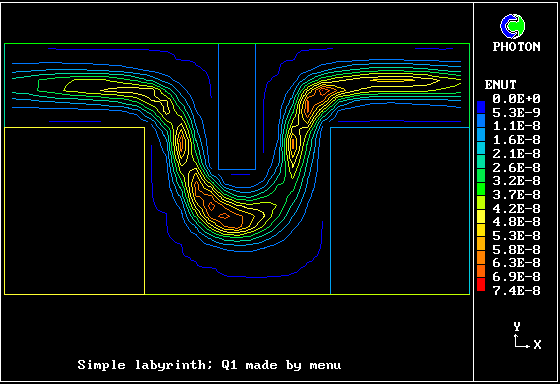
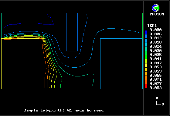
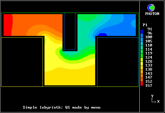
show the distributions of:-
They show further that the results are as good as those of more- widely-publicised models which are much more expemsive to run.
The problem in question is as follows.
The two steel blocks are uniformly heated. The problem is to compute the maximum temperature within the solid at various rates of flow of air.
********************************************************************
*                                                                  *
*       ///////////////////////////////////////////                *
*       --------------- adiabatic wall ------------                *
*   --->                   duct                    ----->          *
*       -------------                 -------------                *
*       // steel ///|     cavity      |/// steel //                *
*       -------------------------------------------                *
*       ////////////// aluminium //////////////////                *
*       -------------------------------------------                *
*                                                                  *
* Fig.1  Horizontal dimension 3 cm, vertical dimension 1.2 cm      *
*        The two steel blocks and the cavity are each 1 cm wide.   *
*        The blocks, the aluminium base and the air-flow duct      *
*        are each 0.4 cm thick.                                    *
*                                                                  *
********************************************************************
Predictions were made, with the above-indicated input data, by activating three of the low-Reynolds-Number models which are supplied as standard in the PHOENICS computer code, namely:
Four different uniform computational grids were used, namely:
(a) 6 * 6 ; (b) 15 * 15 ; (c) 30 * 30 ; and (d) 60 * 60 .
Only the last of these can be regarded as likely to provide grid- independent results.
However, the coarser grids are still interesting because, as has been explained above, they are much more likely to represent the numbers of cells which can be devoted to flow elements such as are shown in Fig.1, when these form parts of much larger assemblies.
The results, in the next table, show LVEL to be in fair agreement with the other models for all grid finenesses and Reynolds numbers; and to be much economical.
------------------------------------------------------------------
| Table 1. Maximum temperature rises in the metal, in deg Celsius|
------------------------------------------------------------------
|  Re  grid lvel  2-layr lam-br  |   Re  grid lvel 2-layr lam-br |
|--------------------------------|-------------------------------|
|  100  a  12.96  12.98  13.01   |  1000   a  8.66  7.90   8.76  |
|       b  17.15  17.32  17.40   |         b  5.03  5.03   5.70  |
|       c  17.43  17.61  17.32   |         c  4.04  4.32   5.12  |
|       d  17.57  17.76  17.84   |         d  4.62  4.97   6.01  |
|                                |                               |
|  200  a  12.40  12.43  12.32   |  2000   a  6.58  5.72   6.13  |
|       b   8.81   9.13   9.28   |         b  3.61  3.57   4.32  |
|       c  12.58  12.93  13.18   |         c  2.89  2.62   3.80  |
|       d  12.75  13.12  13.36   |         d  2.70  2.82   3.61  |
|                                |         ----------------------|
|  500  a  10.84  10.65  11.11   |  Computer times for attainment|
|       b   6.39   6.67   7.03   |  of steady state to within 1%,|
|       c   6.26   6.82   7.36   |  in minutes on a Pentium 200  |
|       d   7.90   8.27   9.01   |   2000  d  .lt.1     10 .gt.10|
------------------------------------------------------------------
The computer times in the bottom right-hand corner of the table were deduced by visual observation of the PHOENICS "graphical monitor", and should therefore be taken as approximate.
The .gt.10 entry for the Lam-Bremhorst model appears because oscillations of maximum temperature of amplitude in excess of 1% were still continuing at the 10-minute mark, and seemed likely to continue.
Generally, convergence was more difficult to procure for the Lam-Bremhorst model than for the other two.
The differences between the predictions of Lam-Bremhorst and two- layer models are indicative of the doubts which attach to the credibility of even well-validated models, when they are used for geometries which differ from those for which they have been tested.
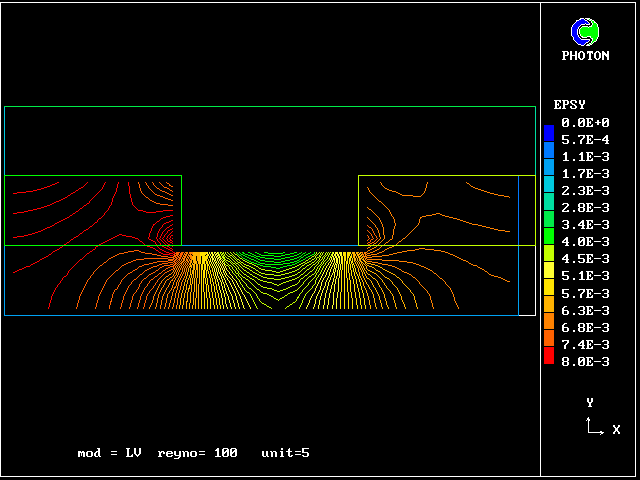
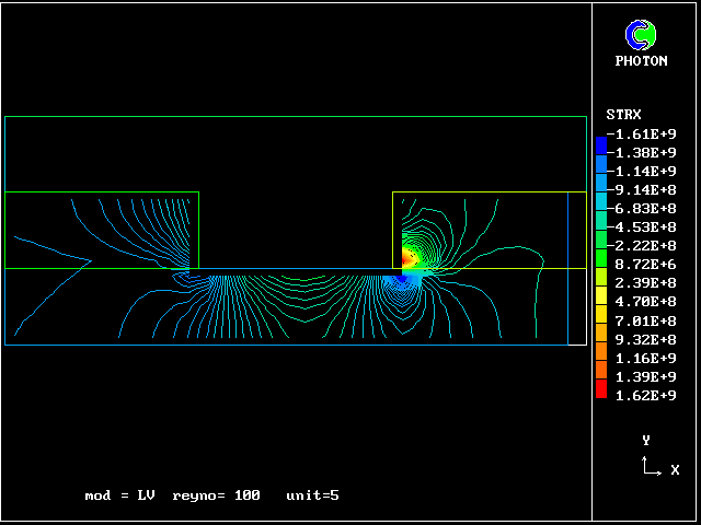
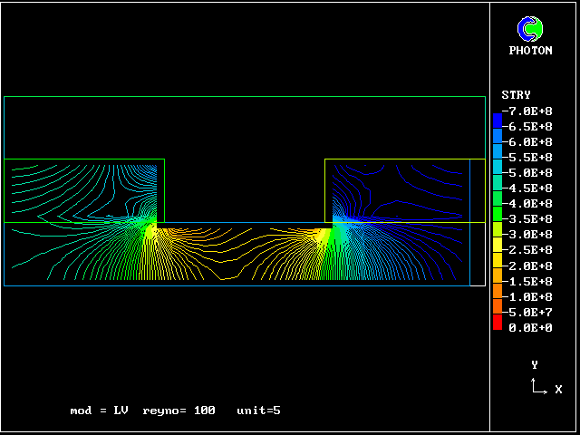
The geometry is similar to that of the previous example; and LVEL is the turbulence model used.
The stresses-in-solids option of PHOENICS has been activated (See PHENC entry: Stress and strain in solids)
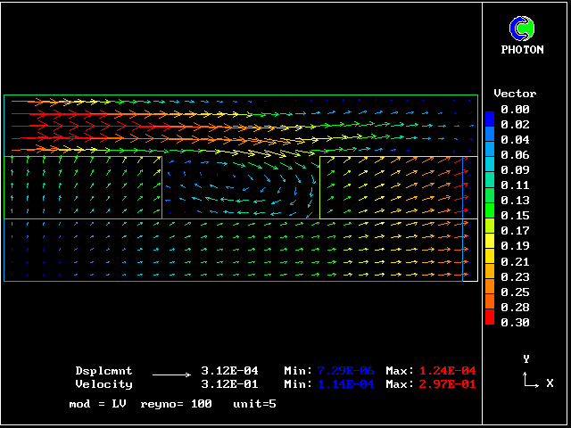
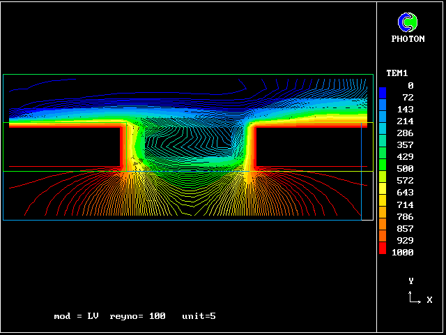
The following picture shows two sets of vectors, namely:
(1) the velocity vectors in the air, and
(2) the displacement vectors in the solid.
Both sets of vectors were calculated by PHOENICS at the same time.
This is possible because the "SIMPLEST" algorithm works for stress and strain in solids just as well as for fluid-flow simulation.
The solids are supposed to be fixed at the bottom left-hand corner Velocity vectors above, displacement vectors below
The two upper blocks, which were heated, have a higher thermal- conductivity than the plate to which they are fixed.
The temperature field which caused the thermal expansion
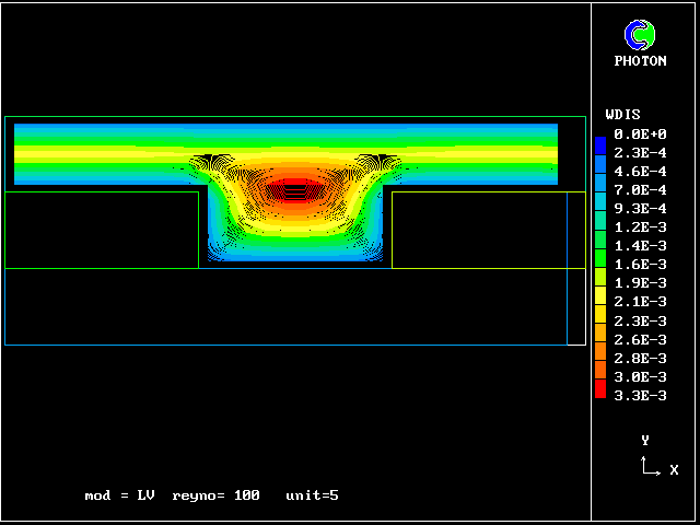
The temperature and flow fields were calculated by means of the LVEL turbulence model, which makes use of the WALL-DISTANCE field computed from a single scalar equation. This is its distribution.
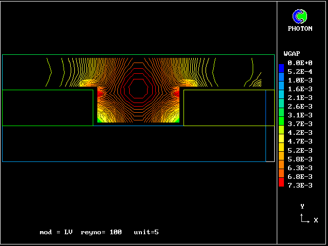
This scalar equation also yields the gap between walls, which is often needed. especially when surface-to-surface radiation is present. Its values are shown here.
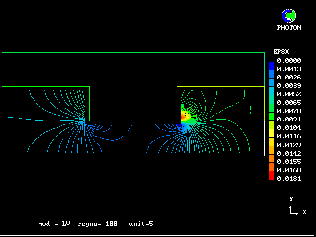
The x-direction strains, deduced from the x-direction displacements. The thermal-expansion coefficients of the plate and blocks differ
The y-direction strains, deduced from the y-direction displacements.
The y-direction stresses
----------- END of the LVEL section ---------
wbs