DIAGRAM 1
with annotations and a new section, in red font, added by dbs in June 2010
X-Cell is a development of the Conservative Low-Dispersion Algorithm (CLDA), which has been attached to PHOENICS for several years. Whereas CLDA was exemplified only for scalar variables, X-Cell applies also to hydrodynamic variables, i.e. velocity components and pressure.
This paper is the first publication about X-Cell. Its aim is to explain the nature of the algorithm, and to report some preliminary results of its use.
Detailed comparison with staggered-grid PHOENICS is made for:
Each of the methods has its advantages and disadvantages.
has been rather little used; and, until version 2.2, it was rather slow to converge.
is the only method to be fully compatible with the multi-blocking and fine-grid-embedding features of PHOENICS; but its convergence has also been rather slow.
All methods employ more computer storage, and more computer time, when the grid is body-fitted.
Note by dbs, June 2010:
Since only two methods are introduced above, what was meant in 1996
by method 3 is unknown; but in 2010 it is no longer important.
BFC grids are most frequently employed when bodies possessing curved surfaces are immersed in the flow; or when the bounding containment walls are themselves curved.
PHOENICS can handle curved-surface situations with Cartesian or polar grids; but finer grids are needed, if the curvature is to be adequately represented, than if a BFC grid is used.
If however, the hexahedral cells employed by PHOENICS could be supplemented by triangular prisms, or pyramids, the task of representing curved-surface bodies in not-too-fine Cartesian grids would be greatly eased.
The X-Cell algorithm, which is the subject of the present paper, appears to be capable of providing the two ingredients required of a superior algorithm; for:
What has resulted is a somewhat unusual formulation, with the following characteristics:-
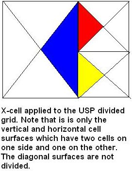
                                          |\-------/|
    The X-Cell grid, the shape of         | \  +  / |
    which explains the name of the        |  \   /  |
    algorithm, can be represented in      |   \ /   |
    two dimensions as indicated on        | +  O  + |
    the right of this text.               |   / \   |
                                          |  /   \  |
    In three dimensions, the triangular   | /  +  \ |
    prisms are replaced by pyramids.      |/-------\|
The X-Cell grid is the same as that of CLDA.
Pressures are stored at the
centre points marked o.
All other variables are stored at
the points marked +.
In general, each six-sided cell
contains six sub-cells adjacent to
the north, south, east, west, high
and low faces.
In time-dependent flows, a further sub-division in the difficult-to-portray time dimension is possible.
The mass fluxes from one sub-cell to another are the same as for CLDA, namely:
                                                      ^
    that from W to N is 0.5*(w + n);             |\---|n--/
                                                 | \  +  /|
    that from N to E is 0.5*(e - n);             |  \ N / |
                                                 w   \ /  e
    that from W to S is 0.5*(w - s); and    +WW-->+W O E+-->
                                                 |   / \  |
    that from S to E is 0.5*(s + e)              |  / S \ |
                                                 | /  +  \|
                                                 |/---^s--|
    Upwind values of all sub-cell variables           |
    are used for the convection terms in the
    balance equations.
In CLDA, the w, n, e and s fluxes were computed directly from the solved-for staggered velocity components.
In X-Cell, w is computed from the distance-weighted mean of the x-direction velocities at sub-cell locations WW and W.
Corresponding weighted-mean formulae are used for n, e, s, and (for 3D) h and l.
                                                       ^
                                                  |\---|n--/
    The diffusion flux between WW and W           | \  +  /|
    is proportional to phiWW - phiW ;             |  \ N / |
    fluxes at n, s and e are computed             w   \ /  e
    similarly.                               +WW-->+W O E+-->
                                                  |   / \  |
    phiO (centre-point value) is then defined     |  / S \ |
    as the weighted averaged of phiW, phi         | /  +  \|
    phiS and phiE.                                |/---^s--|
                                                       |
    The diffusion flux from W to N is computed from the Cartesian
    components proportional to phiW - phiO, and phiO - phiN,
    W, N, S and E being located at the centroids of the sub-cells.

    Computation of associated distances and transport properties
    corresponds in an obvious manner to the above choices
The velocities uNW, uSW, uN and uS all experience momentum sources of one half that value.
The latter velocities all experience further momentum sources from pressure differences which they share with nodes farther west or farther east.
v and w velocities are handled similarly.
Distance-weighting is used for non-uniform grids.
Sources due to chemical reaction, radiation, gravity, ohmic heating and electromagnetic effects are given values proportional to sub-cell volumes.
Turbulence-energy generation terms are computed in the same way as for CCM, with appropriate distribution between sub-cells.
Distributed-resistance momentum sources are given values proportional to cell volumes.
Wall boundary conditions are computed as sources in obvious ways, only the near-wall sub-cell being involved.
All sub-cell values are currently solved point-by-point.
This is a temporary measure, to be replaced by SIVA-like procedures in the next stage of development.
SIVA (= Simultaneous Variable Adjustment) was the favoured Imperial College algorithm until displaced by SIMPLE. It has many merits, and is due for revival.
Pressure is solved whole-field, as in SIMPLE, whereafter the convection velocities (w, n, s, e above) are corrected to ensure continuity satisfaction.
These corrections are shared also between the sub-cell velocities.
The square-cavity-with-moving-lid problem has been solved for the Reynolds number of 400. Heat transfer between the moving lid and the bottom surface has been included.
Uniform grids have been employed, with NX and NY equal to each other and (in successive runs) to 11, 21, 31, 41, 51, 61, 71, 81, 91, and 101.
The number of sweeps used has been sufficient for convergence for all the grids, except possibly that with NX = 101. Several thousand sweeps were used for the larger grids, because the (provisional) point-by-point treatment makes convergence slow.
A selection of the results displayed will first be shown by way of contour and vector plots.
Thereafter some numerical results will be presented, which enable their accuracy to be compared with those provided by the standard PHOENICS algorithm, which employs a sta(1))ggered Cartesian grid.
What will first be shown are the vectors deduced from then mass-flux velocities, followed by contours of longitudinal velocity for each of the sub-cells.
The grid has NX = NY = 21 .

West sub-cell and north sub-cell longitudinal velocity contours
South sub-cell and cell=averaged
longitudinal velocity contours
The following table shows the values of the minimum velocity on the centre line in the lid-movement direction, for various values of NX.
Below the values from the X-Cell solutions are those for standard PHOENICS.
   NX      11    21    31    41    51    61    71    81    91   101
   XCell -.187 -.267 -.302 -.317 -.322 -.329 -.329 -.329 -.3.. -.317
   Stnd. -.149 -.210 -.259 -.285 -.301 -.312 -.317
It should be noted that the X-Cell results for the larger grids may not be completely converged.
The following table shows the values of Nusselt Number for the top wall, times 0.5, for various values of NX.
Below the values from the X-Cell solutions are those for standard PHOENICS.
   NX      11    21    31    41    51    61    71    81    91   101
   XCell   2.28  2.48  2.63  2.61        2.55  2.53  2.64       2.34
   Stnd.   2.15  2.134 2.16  2.25  2.25  2.27  2.28
It should be noted that the X-Cell results for the larger grids may not be completely converged; for the scalar-equation solution procedure, at present, is slower than that of the momentum equations.
Inspection of the table containing minimum-velocity data suggests that:
This is understandable; for the thin boundary near the moving lid is decisive for heat transfer; and the distance from the wall to the nearest sub-cell is one-third for X-Cell of what it is for standard PHOENICS.
One of the potential advantages of the X-Cell algorithm is that it may permit curved-boundary problems to be solved adequately with Cartesian or polar grids rather than body-fitted ones.
Therefore, one of the flow situations which has been chosen for simulation with the aid of X-Cell is the steady flow over a circular-sectioned cylinder.
Of the various cases investigated, results for the following will be presented.
From the successive grid refinements of cases (3) and (4), it is desired to establish how fine a grid is needed for grid- independent solutions to be achieved.
First the 36 * 13 grids will be shown.
Then the velocity vectors, longitudinal-velocity contours and temperature contours will be presented.
Finally the recirculation-length data will be reported, for all three grid finenesses.
The following figures compare the solutions in respect of velocity and temperature fields.
Longitudinal Cartesian velocity contours for the BFC and X-Cell grids


Temperature contours BFC and X-Cell grids, NX*NY = 36*13
The influence of grid fineness on the recirculation length has been found to be as follows:-
| NX * NY | X-Cell | BFC | Measured |
| 27*13 | 2.3 | 1.15 | 2.75 |
| 36*13 | 2.6 | 1.25 | 2.75 |
| 60*30 | 2.8 | 1.5 | 2.75 |
It is evident that the coarsest X-Cell grid produces better results than those from the finest BFC grid.
The work on the square cavity has shown that X-Cell produces more accurate results than standard PHOENICS when both are using upwind differencing.
It is true that higher-order schemes, which are available in the Advanced Numerical Algorithms option of PHOENICS, will improve the staggered-grid solutions, whereas such schemes have not yet been devised for X-Cell.
Nevertheless, the superiority of X-Cell over standard PHOENICS is such that an X-Cell solution is often more accurate than a standard PHOENICS solution with twice the number of cells in every direction; and it also uses less computer storage.
The slowness of convergence of the X-Cell algorithm at the present time has to be admitted; but it is an eradicable and therefore temporary feature.
Many means are available for introducing greater implicitness into the solution procedure; and, now that the inherent accuracy and stability of X-Cell has been established, attention will immediately be given to introducing these means.
PHOENICS has in any case too long suffered the disadvantages of the sequential mode of solving for one variable after another.
For chemical reactions, for multi-phase flow, for advanced turbulence models, and for many other circumstances in which strong interactions exist between different variables associated with the same cell, sequential solution is NOT the best.
X-Cell may provide the stimulus which leads to an appropriate consideration of variable-to-variable links.
The results presented for the circular-cylinder flows are probably even more significant; for they suggest that curved-boundary flows may be computed more accurately with coarse Cartesian X-Cell grids than with BFC grids with greater numbers of cells.
"Suggest" is the right word; for there are many more cases which should be tried before a firm conclusion can justifiably be drawn.
The exploration of a wider range of examples is a matter of great urgency.
Three examples of practical applications of X-Cell will now follow.
Comparisons with experimental data or BFC solutions have not yet been made.
1. X-junction carved in block (NB: PHOTON does not understand the diagonal blockages )
2, The flow in a chamber with inserts of irregular shapes
Most of the examples shown in the present paper have concerned the XY plane; however, X-Cell has been introduced into PHOENICS in a general manner; and tests have shown that the implementation involving the Z-direction is just as satisfactory.
Although X-Cell is easiest to describe for two-dimensional situations, it is valid also for one- and three-dimensional ones.
The following picture shows an example of a three-dimensional calculation, the purpose of which is to illustrate the low- dispersion characteristics of X-Cell, which it inherits from CLDA. The grid is 5 x 5 x 5.
This is an example of low dispersion behaviour of pyramidal Std. PHOENICS solution sub-cells.
- Velocity components are fixed at
U1=V1=W1=sqrt(3)/3
- Step scalar discontinuity X-Cell CLDA solution
along the diagonal plane
The X-Cell algorithm handles without difficulty the transfer of heat from solid to fluid, whether the boundaries are aligned with the main-cell walls or with their diagonals.
PHOENICS has, for several years, been able to compute the displacements (and therefore strains and stresses) within solids immersed in fluids, simultaneously with the velocities, pressures and temperatures which give rise to those displacements.
This capability is incorporated in the solid-stress option of PHOENICS.
The option has been little used, so far; and one of the reasons is that its satisfactory working has been GUARANTEED only for Cartesian grids, whereas potential users have argued that curved surfaces demand body-fitted coordinates.
X-Cell has already been extended to problems in which stresses are solved for in the immersed solids, simultaneously with the velocities, etc, in the fluids themselves.
Because X-Cell is able to represent curved boundaries in Cartesian grids rather successfully, as has been shown above, it may provide what the PHOENICS solid-stress option needs to secure acceptance.
The next two examples are of the solid and stress calculations using X-Cell grids both for fluid flow and solid-in-stress calculations.
On the basis of experience so far, there are good prospects that:
At present, the user of X-Cell is required to introduce commands into the Q1 file which allocate storage for the sub-cell variables, which activate special XCEL and DPXCEL patches, etc.
Such features are appropriate to an algorithm which is under development; but, if X-Cell is to be frequently used, it must suffice for users to insert XCEL=T in their Q1 files.
XCEL=T may indeed become the default setting.
Then the additional storage must be automatically provided; and boundary-condition data which users have supplied as though they were employing a staggered grid must be automatically translated into boundary conditions for sub-cell variables.
At present, X-Cell has been applied only to laminar flows, of which the viscosity and Prandtl-Schmidt numbers have been uniform within the fluid.
Extension to non-uniform fluid properties presents no difficulties; but it remains to be done; and, as is always the way, doing so will necessitate some re-thinking of the methods of computing and using properties within PHOENICS.
Turbulent-flow simulation will require the energy-generation terms to be coded; and wall-function strategies for walls coinciding with cell diagonals will have to be devised.
Two-phase, multi-phase and free-surface features are still to be activated in X-Cell; and chemical reaction, radiation and other processes require to be exemplified.
So many items of engineering equipment are tubular in form that the CARTES=F setting is frequently selected in the Q1 files of PHOENICS.
Even though X-Cell can, it appears, handle curved boundaries rather satisfactorily, it would be perverse therefore to refrain from adapting it to polar-coordinate grids.
The question of whether the sub-cell velocity variables should be those aligned with the grid or remain as the Cartesian components is an open one; and, provided that care is taken in formulating the algebraic equations, the solutions should be the same in both cases.
One special argument favours the choice of the Cartesian components: it would be a useful step on the road to X-Cell-BFC.
Despite the prospect of being able to dispense with BFC grids in many circumstances in which they are currently used, it is to be expected that the requirement for some body-fitting will remain,
For example, flow in a turn-around duct, or in a sinuous tube, will be best simulated by means of a grid which follows the duct or tube shape.
There will therefore inevitably be some pressure to develop a BFC version of X-Cell; and no difficulties of principle appear to stand in the way.
Probably the method will use the Cartesian components as the velocity variables.
Finally it must be recognised that PHOENICS users will have confidence in the X-Cell algorithm only when the validity of the flow simulations which it produces has been extensively demonstrated.
What has been presented here, even augmented by other work which has been done but nor reported, falls far short of what is needed.
The assistance of Mr Nikolay Pavitsky, of CHAM-MEI, in the development of the Fortran coding embodying the X-Cell algorithm, is gratefully acknowledged.
This work has been funded by Concentration Heat and Momentum Ltd.
Although this suspension was then thought of as being temporary, it has in fact lasted until the present day (June 2010).
Many other developments have since 1996 been been attached to PHOENICS, including:
Later, for reasons connected with the easier procurement of convergence, a staggered-grid formulation was employed, which is indeed the currently-preferred method.
The X-Cell formulation, it can now be recognised has the desirable features of both collocated and staggered grids, in that:
If to this is added the low-numerical-diffusion feature afforded by the diagonal splitting of the cells, the adoption of X-Cell for both structured and unstructured PHOENICS appears to be very advantageous.
Several suggest themselves, the most obvious being the use of a conjugate-gradient solver, which can certainly handle all the equations which are involved. However, this may not be the most efficient procedure; therefore some attention should be given to some others, as follows:
Thay is not the only way which may be envisaged. Thus the SIVA (= SImultaneous-adjustment-of-VAriables) method might be adapted in which all the velocities associated with a hexahedral cell are eliminated from the cell's continuity equation by substitution from their momentum equations; then adjustment are carried out systematically and repeatedly over all the cells in the domain until all imbalances are sufficiently small.
This method and others have many variants, published and unpublished. How they well they will work for the unconventional X-Cell situation remains to be investigated.
Whatever solution procedures are investigated, it is probable that use of In-Form will provide the best means of experimentation.
Lastly, since the name X-Cell can be to easily confused with that of the Microsoft Excel program, it will probably be wise to employ a different name for the algorithm (or set of algorithms) to studied.
It is suggested that SIMPLE-X is suitable; and probably the hyphen will soon be omitted.