There has long existed a PHOENICS module called PINTO, the PHOENICS INTerpolation prOgram, which allows large fine-grid simulations to be performed in stages.
At the first stage, a coarse grid is used; then interpolation in the resulting phi file produces a second phi file corresponding to a finer grid.
This file is used as the re-start input to a second-stage calculation; of which the resulting phi-file is again subjected to interpolation and used for a third-stage re-start.
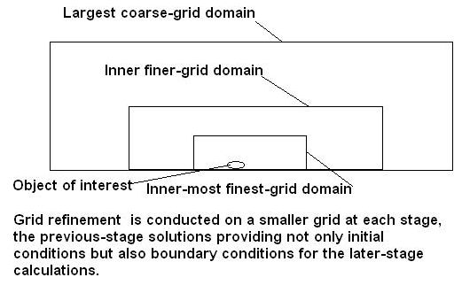
This process continues until the desired finest grid is attained; and the total time of calculation is, if the optimum number of stages is employed, significantly less than if the fine-grid calculation had been started from scratch.
The final converged solution is of course entirely unaffected by the coarseness of the earlier-stage solutions; but it is achieved more rapidly because the finest-grid operation has started from nearly-correct initial fields.
However the original PINTO was unable to handle the large phi-files which are nowadays common in CFD practice.
Further, because PINTO was created well before the introduction of the PARSOL technique, it made no provision for handling the pbcl.dat file, which expresses the extent to which cartesian cells are intersected by objects with curved surfaces.
SPINTO is entirely compatible, it should be mentioned. with parallel-computing operation of PHOENICS.
It can also, as could PINTO before it, be employed for grid-coarsening operations, should be need for coarsening arise.
It can be activated by issuing the DOS command:
runspin
SPINTO then looks for a file, Q1SPIN, containing its instructions; then for a phi file, and, when used for coarsening also for a q1 file, on which to carry them out.
These operations can be those of either refinement or coarsening, for reasons which will be explained below; and the result of SPINTO's speedily-conducted operations is a new phi-format file called NPHI.
Therefore if the user wants to split each cell of grid in X-direction into 2 parts then he should set command REFINE(X,2).
If the user does not want to refine, for example in the X-direction, then he should either use the command: REFINE(X,1) or omit the x-direction command entirely.
NOTE! The ORIGIN command should be used with REFINE commands only.
NOTE! Command SIZE should be used with REFINE commands only.
If the user does not want to coarsen, for example in X-direction, then he should either use the command: COARSE(X,1) or omit the x-direction command entirely.
NOTE! The COARSE command should be used with SAVEGRD commands only (see below).
NOTE! Command USEGRID should be single command besides command STOP (see below).
These commands allow users to test whether it is indeed better to use
interpolation (which sometimes involves extrapolation also) or simply
to place the average values of the coarse cell into each of the finer cells
into which it is split.
Insufficient experience has been gathered so far to indicate which
practice is the better one (if indeed such a general conclusion can be drawn).
NOTE! These commands should be used only in conjunction with REFINE commands.
refine(x,2)
refine(y,2)
refine(z,2)
do not interpolate p1
do not interpolate u1
do not terpolate v1
do not interpolate w1
stop
It is indeed extremely short.
SPINTO allows three methods of working. of which the first two are for users seeking to save computer time, and the third is for use in quality-assurance studies.
If the user wishes to make runs with two levels of refinement, the refinement factor being two-fold in each direction, he should do the following:
Prepare the file q1spin, containing the next lines:
REFINE(X,2)
REFINE(Y,2)
REFINE(Z,2)
STOP
If the user wishes to make the following sequence of operations:
REFINE(X,2)
REFINE(Y,2)
REFINE(Z,2)
ORIGIN(0.1,0.1,0.1)
SIZE(0.8,0.8,0.8)

STOP
Method 2 has not been exemplified below; and indeed experience of using it is not yet extensive.
The underlying idea is that, in circumstances such as are represented by example 4.3 below, in which the region of interest is small in comparison with the whole domain, a coarse grid is quite sufficient for simulating the flow in regions remote from the body; consequently it is only the region which is close to the body which requires refinement.
The third method is useful when the user wishes to be sure that his coarser grids exactly correspond to the finest grid after refinement.
It is especially useful when the grid is non-uniform, being made so, perhaps, to conform with the bounding boxes of VR-objects.
In this case he should make the next sequence of operations.
SAVEFINE
STOP
COARSE(X,2)
COARSE(Y,2)
COARSE(Z,2)
SAVEGRD(COARSE)
STOP
USEGRID(FINE)
STOP
REM The purpose of the script is to enable the advantage gained from the
REM use of SPINTO to be established by obtaining first a non-SPINTO
REM solution corresponding to a single restart (and therefore a total
REM number of sweeps equal to 2*SWEEPS with the solution obtained after
REM SPINTO-using sequence in which PARSOL=T only for the finest-grid run.

REM This file, simple.bat, organises a series of runs in which a coarse grid
REM is refined twice for a Q1 in which there are facetted objects in the
REM domain and PARSOL=t
REM Parsol is set =f for all the coarser-grid runs.
REM
REM LSWEEP is set equal to the environment variable SWEEPS for all runs.

REM the runs are:
REM 1. finest grid, parsol=t, lsweep=2 so as to create pbcl.dat
REM    This may be omitted if facetted objects are absent or if parsol has
REM    been set =f in the original q1

REM 2. coarsest grid, parsol=f,

REM 3. SPINTO restart from run 2, finer grid (*2 in all directions), parsol=f

REM 4. SPINTO restart from run 3, finest grid (*2 in all directions), parsol=t

REM 5. finest grid, non-SPINTO, non-restart, parsol=t
Readers who are unfamiliar with DOS scripts (i.e. 'batch files', should note that only those lines which do not begin with REM (an abbreviation for 'remark') are acted upon.
THe execution of the script starts when 'spinto' is entered at the DOS prompt
REM The q1 is set up with the coarsest grid; and it contains an incl(spinxyz1)
REM statement above its subsequent grid-setting statements.
REM The spinxyz1 file is written by the spinto executable each time it runs;
REM but the spixyz1 files for runs 1, 2, 6 and 7 are written by the present
REM script.
REM The spinto executable also writes a spinxyz2 file. But this is not used.
REM Instead, the present script  puts all necessary additional instructions
REM into the q2 file.
REM The present script also write the Q1spin file which gives SPINTO its
REM instructions.


REM If it is desired to terminate execution of this script at any stage,
REM place the following 'goto end' at the desired location if this file,
REM after first REMoving the 'REM'from in front of it.
REM goto end

REM The following environment variable, SWEEPS, is the number of sweeps
REM to be carried out in all runs
SET SWEEPS=5

REM When the following environment variable = 0, Run 1 is omitted.
REM When it equals 1, Run 1 is carried out
SET PARSOL=0
The environment variables are changed by editing the spinto,bat file; and it is possible to give SWEEPS a different value for each run if that is desired.
PARSOL must be set equal to 1 is facetted objects are to be handled by the PARSOL technique.
echo run started >log
GOTO %PARSOL%
:1
REM Run1, to make pbcl.dat
REM initialization of file INCLuded in the q1 by the statement
REM  INCL(SPINXYZ1)
REM which must appear there immediately after the statement which
REM sets the values of NX, NY and NZ
REM the 4s correspond to the fact that 2 levels of refinement are to
REM be carried out, with refinement factors of 2 in each case
ECHO nx=4*nx; ny=4*ny; nz=4*nz > spinxyz1

REM Perform the first finest-grid run
ECHO TEXT(1 no restart; finest grid; make pbcl >Q2
echo lsweep=2 >>q2
echo run 1 starting >>log
CALL SE
copy pbcl.dat pbcl.sav
echo pbcl saved >>log

:0
REM Run 2, coarsest-grid
REM initialization of file INCLuded in the q1
ECHO    no refinement > spinxyz1
ECHO TEXT(Run 2; no restart; coarsest grid >Q2
echo lsweep=%sweeps% >>q2
echo parsol=f >>q2
REM echo store(prps) >>q2

REM The following settings have no particular connection with SPINTO
REM They over-write those in the original Q1
relax(u1,falsdt,1.0) >>q2
relax(v1,falsdt,1.0) >>q2
relax(w1,falsdt,1.0) >>q2
conwiz=t
echo run 2 starting >>log
CALL SE
echo run 2 completed >>log


REM Prepare for SPINTO runs by echoing the necessary lines to q1spin
ECHO refine(x,2)            >Q1SPIN
ECHO refine(y,2)            >>Q1SPIN
ECHO refine(z,2)            >>Q1SPIN
ECHO do not interpolate p1  >>Q1SPIN
ECHO do not interpolate u1  >>Q1SPIN
ECHO do not interpolate v1  >>Q1SPIN
ECHO do not interpolate w1  >>Q1SPIN
ECHO stop                   >>Q1SPIN
echo q1spin written >>log
REM According to the above commands, SPINTO will double the cell
REM numbers in each direction
REM It also: 1. writes the new values of NX, NY, NZ into the file
REM             spinxyz1, which is INCLuded in the Q1 file before the
REM             grid is created;
REM          2. declares the boolean variable NEWPHI and sets it = T
REM          3. reads the existing PHI file and creates therefrom
REM             a new file, NPHI, from which the next EARTH run restarts.
REM It also writes a file called spinxyz2 which is however no longer
REM INCLuded by the Q1 because its content more visible transmitted by
REM the following lines to the always-read Q2 file.

REM Run 3, the first re-start-with finer grid
ECHO if(newphi) then                      >>Q2
The REMs in front of the PRPS-related statements should be removed if its is desired to call, at the end of the script, for a non-restart run with the finest grid. For then the original fiinit(prps) will be needed.
REM ECHO real(fiinprps)           >>Q2
REM ECHO fiinprps=fiinit(prps)    >>Q2
ECHO restrt(all)                  >>Q2
REM ECHO fiinit(prps)=fiinprps    >>Q2
ECHO namfi=nphi                   >>Q2
ECHO endif                        >>Q2
ECHO TEXT(3  finer-grid restart   >>Q2
echo lsweep=%sweeps% >>q2
REM Call runspin to activate SPINTO, then se for SATELLITE and EARTH,

CALL RUNSPIN
COPY NPHI NPHI3
echo run 3 starting >>log
CALL SE
echo run 3 completed >>log

REM Run 4, the second re-start with still-finer grid
copy pbcl.sav pbcl.dat
ECHO parsol=t                                    >>Q2
ECHO TEXT(4 finest-grid restart parsol=:parsol:  >>Q2
REM Call runspin to activate SPINTO, then se for SATELLITE and EARTH,

CALL RUNSPIN
COPY NPHI NPHI4
echo run 4 starting >>log
CALL SE
echo run 4 completed >>log
:end
For ease of understanding, the above script has been stripped of other statements which it is usually found convenient to include, for example those which save the intermediate results for later study.
There is much which an adept script writer can include which saves himself and others needless labour.
If a long (400-sweep) run is made the graphical-monitor display of the convergence behaviour is as shown below:
Evidently, even after 400sweeps, with an associated computer time of 2283 seconds, the pressure field has not quite converged.
Its contours on the symmetry axis are shown below:
The script, which can be inspected by clicking here causes six 30-sweep runs to be performed as follows:
The symmetry plane pressure distribution is shown below:
It is very similar to that of the 2283-second run. The final graphical-monitor output was as follows:
Evidently small sweep-to-sweep changes in the maximum and minimum variables are still occurring; but it can be concluded that the SPINTO-aided run series has produced a solution which is very nearly as good as that of the 400-sweep non-SPINTO run in less than a quarter of the computer time.
Increasing each of NX, NY and NZ four-fold would improve the accuracy; but the computer time would increase by a much larger factor. Therefore the stage-by-stage coarsening allowed by PINTO may bring some advantage.
This has been investigated in the following manner:-
Here it is seen that the last-sweep maximum and minimum pressure in the domain are 1.29 and -0.575 respectively, and that their last sweep-to-sweep changes were 5.73E-3 and -2.89E-3 respectively.
To judge from the shapes of the red curves, convergence has not yet been reached; but it appears to be close.
The sweep-to-sweep variations of the velocity components are very small.
Here it is seen that the maximum and minimum pressures, namely 1.45 and -0.675 are significantly different from before, and that the final sweep-to-sweep variations are an order of magnitude greater.
It seem reasonable to conclude that the 40-sweep SPINTO-assisted run is of higher accuracy than the 80-sweep un-assisted run.
One may conclude that SPINTO assistance has provided a better solution in little more than half the computer time.
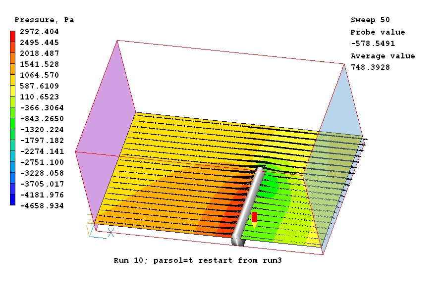
Of special interest is the flow in the immediate vicinity of the obstacle, shown in the following images:
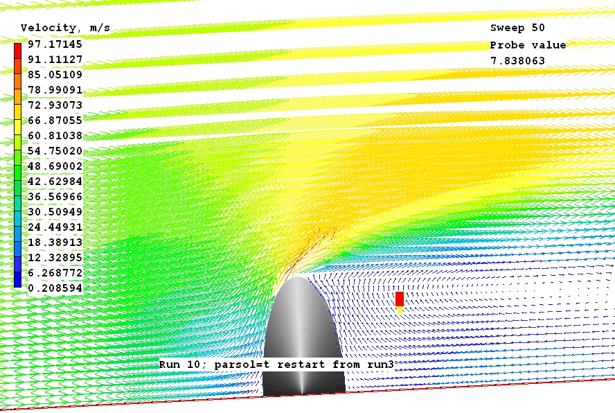
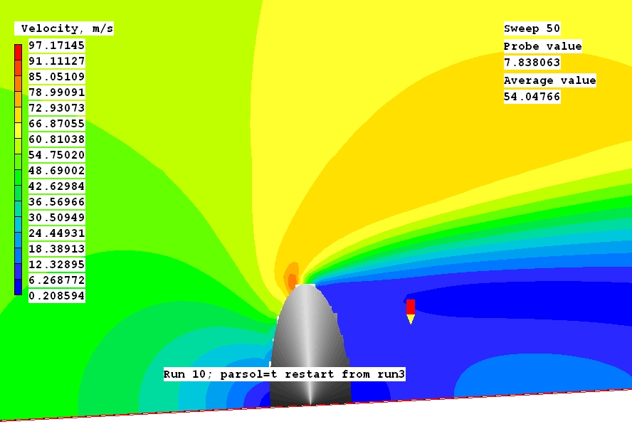
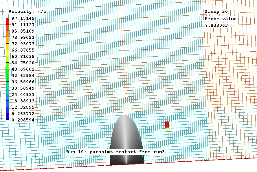
Evidently PARSOL is active.
Many runs were made, both with SPINTO and without; and they showed convincingly that the use of SPINTO both increase the accuracy of the final calculation and significantly reduces the computer time needed to achieve it.
Sufficient proof is afforded by the following images, of which the first is the monitor screen of the fourth of four LSWEEP=50 runs, namely:
The graphical monitor is being used in the whole-domain-maximum-and-minimum mode.
The left-hand box shows that the maximum pressure (red curve), for example, has varied between 2.9E3 and 3.3E3 pascals during the run, and has become 2.97E3 at its end.It has not quite stopped varying; but its change in the last sweep was 2.53E-1 pascals, i.e. less that 0.01 % of the absolute value.
The right-hand box shows that the minimum pressure has also almost settled to an unchanging value, its latest change being even less than that of the maximum pressure.
Inspection of the curves and values pertaining to the other variables gives a similar impression of near-convergence.
The computer times of the four runs were: 2, 9, 36, and 184 seconds respectively. i.e. 231 in total.
Those results were achieved by the use of SPINTO. Now let us examine the final monitor displays of a 400-sweep run in which SPINTO was not used, shown below.
At first glance it might appear that the convergence is not bad; for the right-hand halves of the red curves appear to be nearly horizontal. However this is explained by the fact that the ranges (i.e. differences between 'low' and 'high') are much bigger than before.
Inspection of the corresponding last-change values show that the domain-minimum values of pressure are still changing at the rate of 1.96 pascal per sweep; and that the minimum pressure (-5.26E3) is still a long way from the -4.66E3 pascals shown in the previous calculation.
It is therefore justifiable to claim that the 50-sweep 'spintoed' run gave a better solution than the 400-sweep run which did not use SPINTO.
Moreover the computer time for the latter was 1723 second, i.e. more than 7 times that of the total of all four runs of the SPINTO-using calculation.
There are many variants which have not yet been tried. This document must therefore be regarded as a report on work in progress.
Information about the experiences of others who experiment with SPINTO will be gratefully received by the authors.