MFM reproduces the results of FLM when:-
However, whereas FLM requires limitations 1, 2 and 3, and is tied to a particular distribution formulation, MFM is free from these restrictions.
These points are explained and illustrated by way of computations for a "well-stirred reactor".
A convenient way of introducing the laminar-flamelet model (FLM) of turbulent combustion [Refs 1, 2, 3, 4, 5, 6, 7] is as a refinement of the "eddy-break-up" model (EBU) [8]. The latter, first published in 1971, involved regarding a turbulent burning mixture as comprising inter-mingled fragments of just two gases, namely:
It was recognised that, at the interfaces between the two sets of fragments, thin layers of gas in various stages of incomplete combustion must exist; but the fraction of the total volume occupied by these gases was regarded as much less than unity; and the only important consequence of their existence was the primary chemical transformation (fuel + air --> products) which took place in them.
The rate of that transformation, per unit volume of the total
space, was treated as being governed, however, by the rate of
turbulent micro-mixing, for which the quantity:
Here, epsilon represents the volumetric rate of dissipation of the kinetic energy of turbulence, and k the kinetic energy itself.
Although the eddy-break-up model has proved rather successful in predicting overall combustion rates, its total neglect of the chemical kinetics has disbarred it from simulating secondary but important kinetically-controlled processes, such as NOX production in flames.
(b) The FLM
Whereas the EBU pays scant regard to the interface layer between the burned and unburned gases, the FLM concentrates attention upon it; and one of its major concerns is to compute the magnitude of the area of this interface per unit volume: sigma.
The underlying notion is that, if sigma is known, then the
volumetric rate of combustion omega should be capable of
being computed from:
The attractiveness of this idea is that values of Ulam are often known from measurements on Bunsen burners, and similar laboratory devices; and their presence in the formula provides comfort to the combustion specialist for whom the uncertainties of turbulence are somewhat bewildering.
Numerous proposals have been made for the terms in a "sigma-transport equation". A review is to be found in Reference 7. Although they differ in detail, all contain, directly or indirectly, the epsilon / k term of the EBU; for they all have to conform to the experimental facts which that overall-rate term expresses.
The quantity Ulam is also to be found in them, in a secondary role; but recognition that the composition distributions in the interface are unlikely to be exactly the same as in laboratory-measurement circumstances has caused some authors to multiply Ulam by a (sometimes only-vaguely defined) "stretch factor".
The present purpose is not to enumerate the differences between the various proposals or to prefer one to another; instead it is to draw attention to the physical concept which unites them, both with the EBU and with the MFM.
(c) The unifying concept: the "brief encounter"
The following diagram will serve to focus attention on what the models have in common; for it shows, in idealised manner (ie with neglect of all the actual geometrical convolutions), a volume in which two materials, A and B, are separated by an interface of small but finite thickness.
For EBU and FLM, A is unburned gas and B is burned gas (or vice versa). MFM allows more possibilities; but it reduces to the same when EBU- or FLM-favouring conditions prevail.
     Figure 1. Two fluid "blocks" in contact

     --------------------------------------
     .                      / /           .
     .                      / /           .
     .                      / /           .
     .                      / /           .
     .         A            / /    B      .
     .                      / /           .
     .                      / /           .
     .                      / /           .
     .                      / /           .
     --------------------------------------
                             ^
       The interface layer __i
The diagram represents conditions at a particular instant; and all model makers agree that:
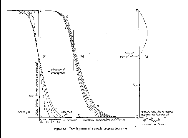
Part (b) shows how, after some time, reaction within the thickened layer causes propagation to occur, finally with uniform speed and layer thickness, into the unburned gas.
Part (c) shows the reaction-rate (plotted horizontally) versus temperature (plotted vertically on the same scale as parts (a) and (b)), which was used as the input to the calculation.
Recognised either explicitly (in MFM) or implicitly (in FLM) by the various model makers is that contact between the A and B "gas blocks" is intermittent, which is to say that, as a consequence of the turbulence, two such blocks:
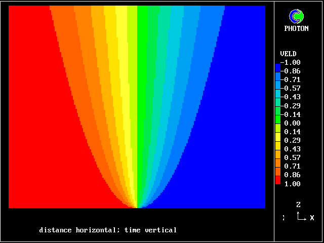
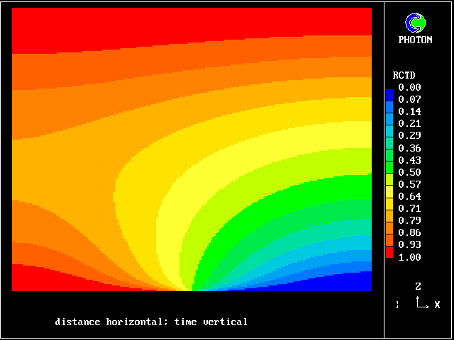
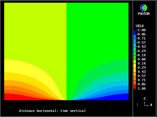
Such a process is nowadays easily subjected to numerical analysis, the results of which may be represented as in the following colour plot.
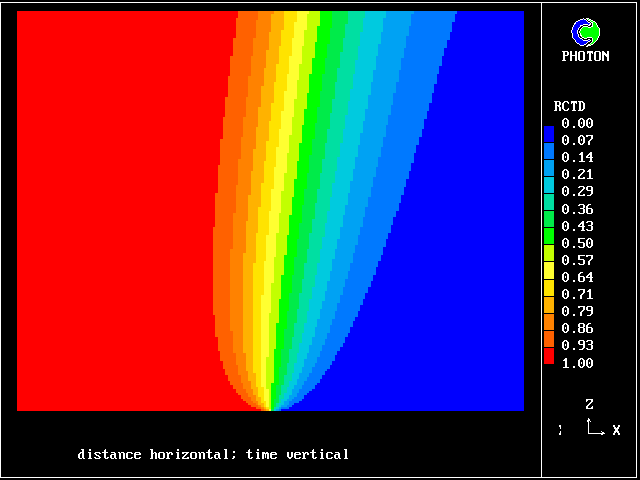
What is noticeable is that the contours are symmetrical at early times, during which interdiffusion domiminates; and they become unsymmetrical later, when chemical reaction "catches up", just as was predicted by the old calculations of Figure 2.
The calculations were performed with the PHOENICS computer code, by the loading of library case 103 .
As will be explained in more detail below, it is the intermittency of these "brief encounters" which explains how volumetric reaction rate comes to be so closely connected with epsilon / k
It will also be shown that the brevity of the contact is such that, at the high Reynolds numbers that are commonly encountered, the interface layer must always be much thinner than the typical block size.
(d) The secondary reactions
Why FLM is superior to EBU is not that it is able to predict better the volumetric rate of progress of the main combustion reaction; for it is doubtful whether it can do this more often than not in circumstances of practical interest.
Its superiority lies in the fact that, through being able to estimate the distributions of the temperature and of chemical species within the interface layers, it allows calculation of the effects of secondary reactions such as those giving rise to oxides of nitrogen.
As will be shown, MFM offers the same possibilities; and in more general circumstances; and, if care is taken to ensure that comparable chemical-kinetic and transport-property presumptions are made, there is no reason why MFM should not produced the same results as FLM, for conditions for which the latter is valid at all.
(a) MFM fundamentals
The multi-fluid model of turbulence has been described in numerous recent publications [10 to 20]; and most of these, and other explanatory material, can be viewed on CHAM's web-site: www.cham.co.uk. MFM is also available for activation in the PHOENICS computer code.
Here, therefore, only the main relevant ideas will be reviewed, as follows:
(b) Connexions with conventional turbulence-modelling concepts
The well-known epsilon and k quantities have already been referred to. It will be useful also to connect MFM concepts with three others, namely:
These quantities are inter-related by equally well-known relationships, namely:-
Since sigma has the dimensions of 1/length, being a measure of the average thickness of the gas fragments engaging in the coupling-and- splitting process, it can be expected to be proportional to the reciprocal of Lmix,
Therefore, to avoid having to introduce another constant, let it be taken as equal to this reciprocal, so that
It is necessary to distinguish between the sigma employed in the FLM from that which is employed in MFM; for FLM pays attention only to interfaces between fully-burned and fully-unburned gases; whereas MFM recognises that the coupling-and-splitting process is a consequence of the turbulence, which disregards the chemical compositions of the materials which are brought into contact.
Thus FLM's sigma has to be zero when there is no more unburned combustible; whereas MFM's sigma can reasonably be taken as inversely proportional to Lmix, regardless of the extent of the reaction.
It is now interesting to ask two questions, namely:
First, however, it is necessary to justify the linkage of the rate of offspring production to epsilon / k by a more detailed discussion of the energy-dissipation process than has been provided anywhere in the MFM literature until now.
(c) The mechanism of energy dissipation
If, as MFM supposes, the dominant behaviour pattern of the multi-fluid population is "coupling and splitting", it must be possible to use this description to explain how turbulent kinetic energy is dissipated. Such a use of the concept now follows.
Obviously, this velocity difference is related to the turbulent kinetic energy by:
It is interesting to observe that such comparisons of MFM predictions with experiment as have been made so far have favoured a value of between 5.0 and 10.0 for CONMIX
The value most favoured by users of the Eddy-Break-Up model, is much lower, namely around 0.5; but this is easily explained by the fact that EBU is a mere "two-fluid" model, i.e. one with a very coarse "population grid".
(d) The average contact time
Since the interfacial layer grows as a result of molecular action, it is certain that its maximum thickness Llay (i.e. that which exists at the end of the "brief encounter" when "coupling" gives way to splitting) is of the order of (nulam * Tcont) ** 0.5 .
Also, the same analysis would show that the rate of production of interface material per unit volume is equal to:
It follows that:
Let now this contact time be compared with the "micro-mixing time", Tmix, defined by:
It follows that, since Re is usually much greater than unity in a turbulent flame, the contact time is much smaller than the mixing time.
One implication is that the interfacial layer does not have enough time to grow so as to have a dimension comparable with those of the "blocks" of fluid which are enjoying their brief encounter. Indeed, it can be algebraically deduced from the above equations that:
It has been remarked above, in connexion with
Obviously the relevance of the epsilon/k quantity to the creation of interface material is greater if the encounter is broken off before the reactedness profile has become very unsymmetrical, i.e. before the laminar-flame propagation process has had time to dominate; so it is interesting to estimate whether this condition is likely to be satisfied.
The following argument allows this question to answered:-
The following summarising remarks about the connexions between FLM and MFM therefore appear to be appropriate:
MFM also has a presumption about the profiles in the layer, as part of its coupling-and-splitting hypotheses. The only presumption which has been seriously explored so far, namely the "promiscuous Mendelian" one, implies symmetry within the inter-diffusion layer; but this can easily be remedied.
FLM requires, for validity:
These requirements are satisfied by PHOENICS Input-Library Case, L103, of which the descriptive part runs as follows.
  Stirred reactor with a 1D population distribution, and
  reactedness, ranging from zero to 1, as the population-
  distinguishing attribute.
                                                    ___________
  It is supposed that two streams of fluid         |           |
  enter a reactor which is sufficiently       A ====>          |
  well-stirred for space-wise differences          |  stirred  |
  of conditions to be negligible, but not          |  ///|/// C===>
  sufficiently for micro-mixing to be              |  reactor  |
  complete.                                   B ====>          |
                                                   |___________|
  The two streams have the same elemental
  composition; but one may be more reacted than the other.

  The flow is steady, and the total mass flow rate per unit volume
  is 1 kg/s m**3 .
The flow is zero-dimensional in the geometrical sense; but, to give it significance for a three-dimensional combustor simulation, it might be regarded as representing a single computational cell in the 3D grid. Then the conditions in the inlet streams might represent those in the neighbouring cells, from which material enters by way of diffusion and convection.
The calculations to be reported have been conducted with a 25-fluid model, and with reactedness as the population-defining attribute.
The reaction-rate-versus-reactedness formula is of the well-known kind:
where R stands for reactedness.
The exponent, CONREA2, has been given the value 5.0, which represents sufficiently well for the present illustrative purposes the temperature dependence of combustion reactions.
Stream A has been chosen as being completely unburned (R=0.0) and stream B as fully reacted(R=1.0).
Various values have been chosen for the micro-mixing constant
CONMIX and
the "pre-exponential factor" of the reactivity, CONREA2
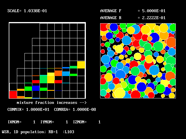
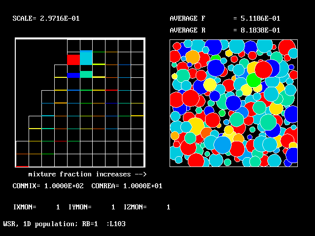
2.2 The PDFs predicted by MFM
In the following table, the second, third and fourth columns disclose the input parameters.
Clicking on the number in the first column will display:
The PDFs appear as histograms, with:
The references to "spikes" should be noted. Comparison of the values ascribed to the height of these spikes with the also-printed "maximum ordinates" shows that they are often much larger. This is the justification for the "two-fluids-mainly" idea which underlies FLM.
The average-reactedness and RMS-deviations appear in the fifth and sixth columns.
| Figure | CONMIX | CONREA | RB | ave. R | rms. R |
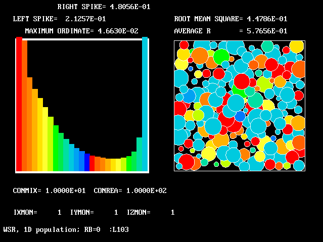 6 6 |
10.0 | 100.0 | 0.0 | 0.577 | 0.448 |
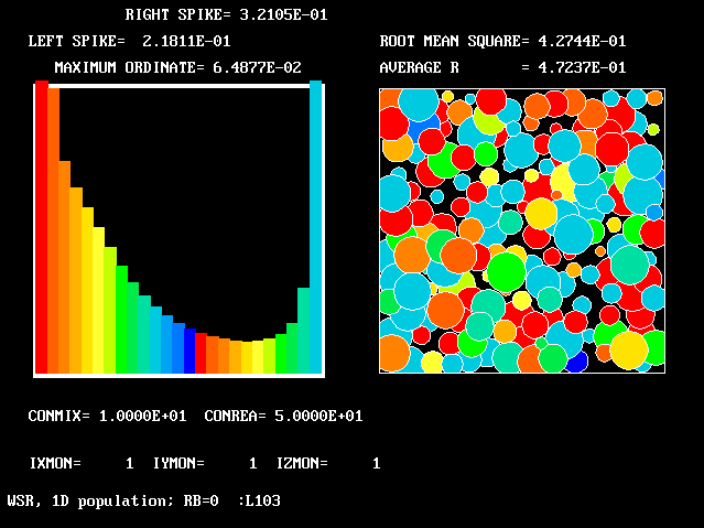 7 7 |
10.0 | 50.0 | 0.0 | 0.472 | 0.427 |
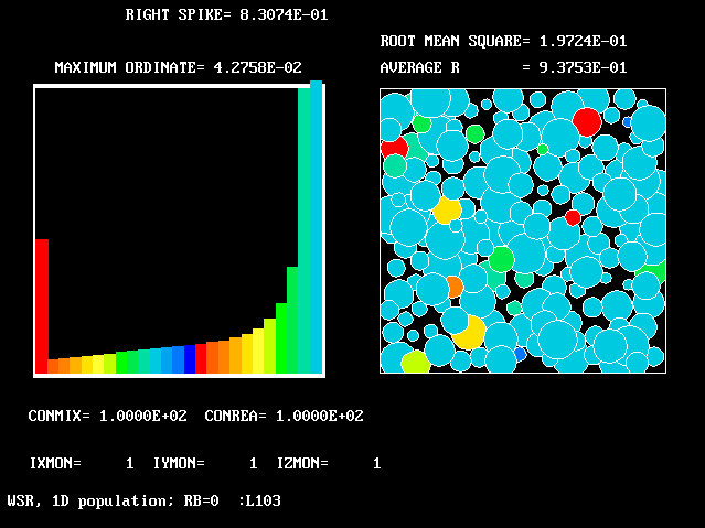 8 8 |
100.0 | 100.0 | 0.0 | 0.937 | 0.197 |
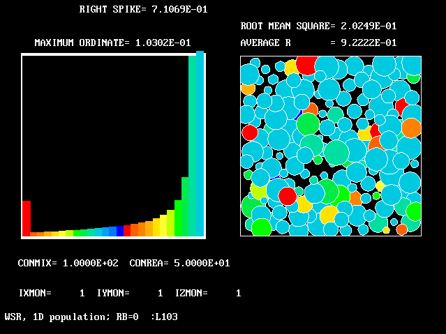 9 9 |
100.0 | 50.0 | 0.0 | 0.922 | 0.202 |
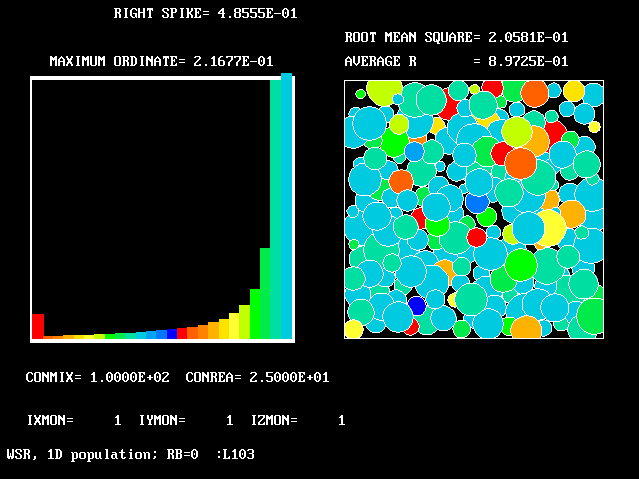 10 10 |
100.0 | 25.0 | 0.0 | 0.897 | 0.206 |
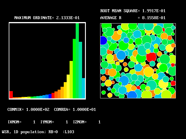 11 11 |
100.0 | 10.0 | 0.0 | 0.815 | 0.199 |
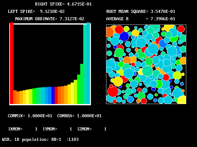 12 12 |
10.0 | 10.0 | 1.0 | 0.739 | 0.354 |
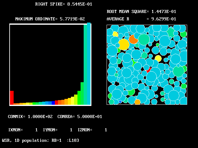 13 13 |
100.0 | 50.0 | 1.0 | 0.963 | 0.145 |
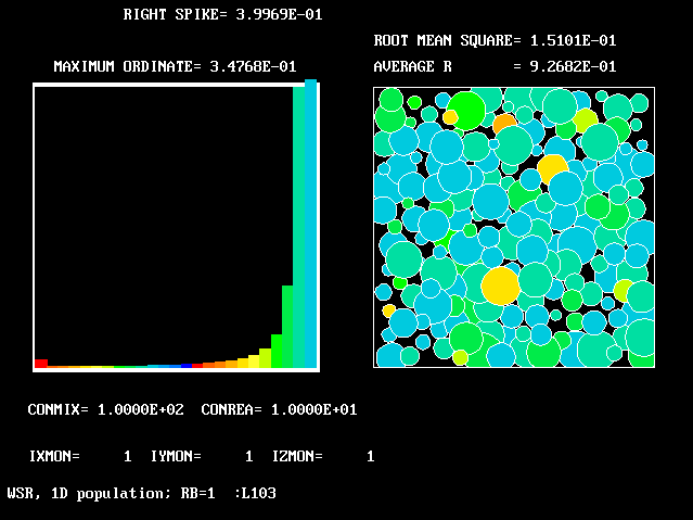 14 14 |
100.0 | 10.0 | 1.0 | 0.927 | 0.151 |
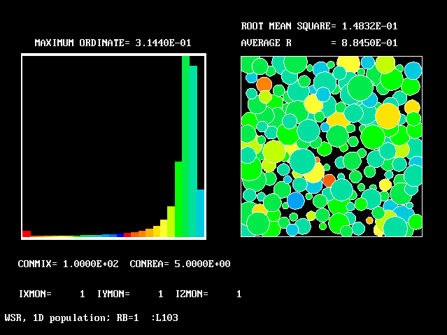 15 15 |
100.0 | 5.0 | 1.0 | 0.884 | 0.148 |
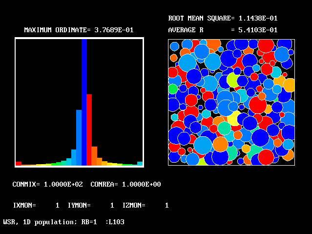 16 16 |
100.0 | 1.0 | 1.0 | 0.541 | 0.114 |
Some trends revealed by these figures will now be discussed, as follows:
In all four cases however, at least one of the spikes is large.
Any further reduction of CONREA leads, it should be mentioned, to extinction of the chemical reaction.
Understandably, the average reactednesses, for the same CONMIX and CONREA, are greater than for the RB=0 flames.
It is now possible to consider to what extent MFM confirms or contradicts the presumptions of the flamelet model of turbulent combustion.
The best confirmation of FLM presumptions is afforded by Figures
Whether the distributions of concentration of the intermediate gases is the same, for MFM and LFM, is another matter. As has already been indicated, LFM practitioners are inclined to believe (albeit without any closely-reasoned argument) that the distributions correspond to those of a steadily-propagating flame; whereas the foregoing analysis suggests that the transient-interdiffusion model is more appropriate.
When the sequence of Figures
Even less supportive are Figures
It must indeed be concluded that FLM can be expected to represent turbulent combustion in pre-mixed gases only when the chemical reaction rate (measured here by CONREA) is large compared with the micro-mixing rate (measured by CONMIX).
This condition is perhaps satisfied for a gasoline engine, where the fuel/air ratio may be close to stoichiometric throughout; but it is unlikely to prevail for combustors into which the fuel and air enter separately.
Separate introduction of fuel and air is the subject of the next section.
(a) The cases considered
A further series of calculations has been performed for the conditions in which the two streams of fluids entering the stirred reactor have differing fuel-air ratios. Such conditions lie beyond the capabilities of the flamelet model at the present time.
Specifically, stream A has been taken as pure air; and stream B has been taken as having a fuel/air ratio of twice the stoichiometric value and a reactedness of 50 %. The two streams are equal in flow rate.
A 100-fluid model has been employed for this study, with a two-dimensional "population grid", of which the PDAs (ie population-defining attributes) are:
Further information about the definition of the model will be provided during the discussion of the results and of their displays, which may be inspected by clicking on the relevant number in the left-hand column of the following table.
| Figure | CONMIX | CONREA | average F | average R |
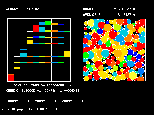 |
10.0 | 10.0 | 0.510 | 0.649 |
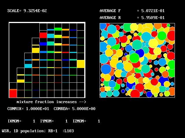 |
10.0 | 5.0 | 0.507 | 0.595 |
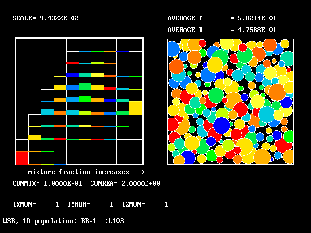 |
10.0 | 2.0 | 0.502 | 0.476 |
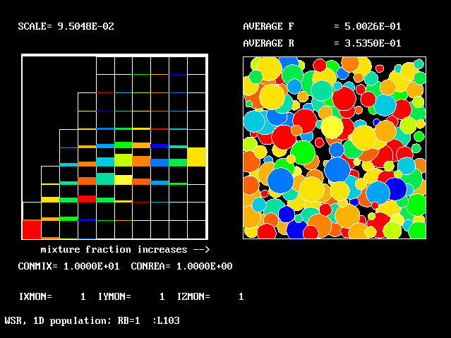 |
10.0 | 1.0 | 0.500 | 0.354 |
 |
10.0 | 0.0 | 0.500 | 0.222 |
 |
100.0 | 10.0 | 0.512 | 0.818 |
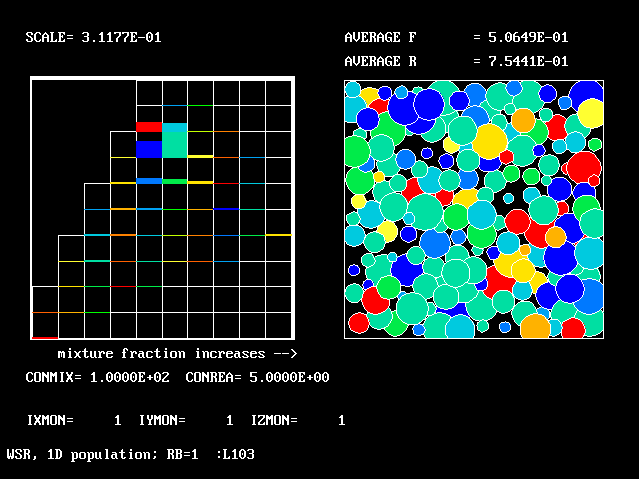 |
100.0 | 5.0 | 0.507 | 0.754 |
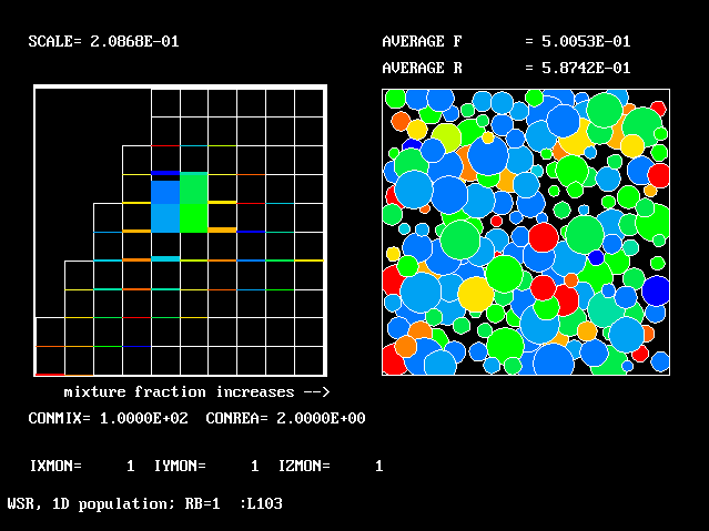 |
100.0 | 2.0 | 0.500 | 0.587 |
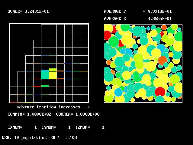 |
100.0 | 1.0 | 0.500 | 0.346 |
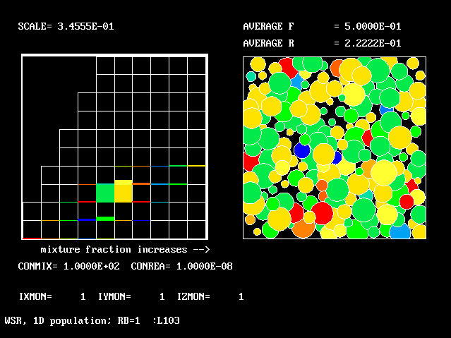 |
100.0 | 0.0 | 0.500 | 0.222 |
(b) Conclusions from inspection of the table
The runs conducted fall into two groups. The first five have the fixed CONMIX value of 10.0, and successively smaller CONREA values; and the next five have CONMIX = 100.0, and the same sequence of CONREA values.
It can be seen that:-
(c) Conclusions from inspection of the figures
All the figures have the same general form. They show a two-dimensional histogram on the left, and a graphical representation of the multi-fluid-model concept on the right.
The latter is similar to that of earlier one-dimensional population distributions; but the average-R value is printed, not the RMS deviation of F.
The left-hand diagram is however quite different from before; for it has to represent the proportions in which the total amount of material is distributed between ten fmx and ten fbu intervals.
"Spikes" no longer make any appearance.
The most-prevalent fluids are those whose "boxes" are most full of colour; the least-prevalent are those whose boxes are black.
The figures will now be discussed individually, in some detail.
When the sequence of Figure 18 to 21 is considered, it is seen that the upper (higher-reactedness) boxes are less-and-less well filled, until, when CONREA has been reduced to zero, for
Indeed, were the "population grid" finer, the histogram would provide colour only along that line.
It will have been noticed that, in all the histograms, boxes lying
to the left of the stream-A-to-stoichiometric-mixture line are
absent.
The reason is that the states represented by such boxes are not
physically attainable; for they correspond reactednesses which
exceed unity.
Therefore, although it has been stated above that a 100-fluid model is in use, the statement is a slight exaggeration; for the concentrations of fluid in the "missing boxes" are necessarily zero, and so need not be computed.
(d) Comparison between FLM and MFM for the cases considered
The above heading is included for, completeness; but there is little to say, for the simple reason that FLM, like the eddy-break-up model (EBU) to which it is the successor, is silent about mixtures of differing fuel-air ratio.
It is however worth emphasising that the "brief-encounter" model, which some writers on FLM appear to grasp, does supply the means by which "flamelet-like" concepts can be applied to turbulent diffusion flames; and it is of course the Multi-Fluid Model which provides the unifying mathematical framework.
As was mentioned at the start of the present paper, FLM is acknowledged by its proponents as being restricted in its validity to the circumstances in which the reactivity of the combustible mixtures is sufficiently high, in comparison with the turbulent mixing process, to ensure that the sum of the volume fractions of fully-burned and fully-unburned gases is close to unity.
In respect of pre-mixed (i.e. uniform-fuel/air-ratio) gases, section 2.3 has confirmed the correctness of this acknowledgement; and it has indicated that MFM permits prediction of combustion processes for which the high-reaction-rate condition is not satisfied.
When combustion of non-pre-mixed gases is in question, of the kind treated in section 3.1, the condition is hardly ever satisfied; for the "brief encounters" result in the creation of interfacial layers in which, perhaps, in some central region, the mixture ratio is near stoichiometric so that the gases are highly reactive. This must however surely be very rare; both in space and time.
It therefore appears proper to conclude that the restriction of FLM to high-reactivity conditions is a very severe restriction indeed.
The third of the limitations to which FLM is subject is that the Reynolds number must be high. This is true of MFM also, as it has been developed so far; but it is interesting to consider which of the models has the better prospect of breaking free from the limitation.
Proponents of FLM have not, to the author's knowledge, pronounced explicitly on this matter; and it is not for him to speak for them. But the following can be said from the MFM side:-
The foregoing discussion may be held to justify the following conclusions:-