FLAIR Tutorial 8: Flow over Big Ben

This is a 3D simulation of the flow over Big Ben. The case is to show how to import the STL of the Big Ben into the FLAIR VR-Editor. The size of the Big Ben used in the simulation is 6m long, 6m wide and 30m high whereas the size of the calculation domain is set to 100m long, 100m wide and 50m high as shown in the picture below. This tutorial is also shows how to use a Wind_profile Object to describe the wind profile at the upstream boundary.

Setting up the model

Start FLAIR with the default mode of operation

• Click FLAIR icon (a desktop shortcut created by the FLAIR installation program); or
• Start the VR-Editor by clicking on 'Start', 'Programs', 'FLAIR', then 'FLAIR-VR'. The VR screen shown in Fig. 2 should appear.
• Click on the 'File' button and then select 'Start new case', followed by 'FLAIR' and 'OK'.

The FLAIR VR-Environment screen should appear, which shows the default domain with the dimensions 10mx10mx3m.

Resizing the domain

• Change the size to 100m in x-direction, 100m in y-direction and 50m in z-direction on the control panel.
• Click on "Reset" button, on the movement panel and then click "Fit to window".

Adding the object to the calculation domain

a. add Big Ben

The geometry of the Big Ben object is available in an STL file. The following steps show how to use the 'Object management' dialog box to import the STL file.

• Click on the 'Object' pull-down menu and select the 'New' (New Object) option on the 'Object management' dialog box to bring up the 'Object specification' dialog box
• Change name to 'BIGBEN'.
• Click on the 'Place' button and set 'Position' of the object as:

X: 40.0 m

Y: 40.0 m

Z: 0.0 m

• Click on 'Shape' button. This will bring up the 'Shape' dialog box as shown below

• Click on the Import CAD geometry from 'STL File' button. This will bring up a 'Open file' dialog box, initially diaplying STL files in the working direction.
• Locate the bigben.stl in the directory /phoenics/d_intfac/d_cadpho/d_stl as shown below

• Click on 'Open' button to load the bigben.stl file. The 'Import STL data' dialog will appear on the screen as shown below

• Clicking 'OK' will bring up the 'Geometry Import' dialog box as shown below
• Toggle 'Take size from Geometry file' button to 'Yes'. This will enable you to make 'CAD X Y Z align with VR coodinates. In this case, the original size shows that the upright direction is Y in the original geometry file (dy = 28.5m) and it should be align with the Z direction (upright) in FLAIR-VR. So we set 'CAD X Y Z align with VR 'Y Z X'.

• Click on 'OK' to convert the import STL file to the VR data file, bigben.dat
• Click on the 'Size' button and set 'Size' of the object as:

X:6.0 m

Y:6.0 m

Z:30.0 m

• Click on 'OK' to close the 'Object specification' dialog box.

b. create the inlet boundary with a wind profile

In order to create a wind profile, we use a User-defined object combined with the In-Form facility.

• Click on the 'Object' pull-down menu and select the 'New' (New Object) option on the 'Object management' dialog box to bring up the 'Object specification' dialog box
• Change name to 'IN'.
• Click on the 'Size' button and set 'Size' of the object as:

X:100. m

Y:100. m

Z: 0. m

• Click on the 'Place' button and leave the default 'Position' of the object as:

X: 0.0 m

Y: 0.0 m

Z: 0.0 m

• Click on 'General' and select 'Wind_profile' from the object 'Type' list.
• Click on 'Attributes' button. The dialog shown below should appear on the screen

• Set the X-direction velocity component to 3.0 m/s
• Set the reference height to 5.0 m
• Click on 'OK' to close the 'Wind profile Attributes' dialog box
• Click on 'OK' to close the 'Object specification' dialog box

c. add the sky

• Click on the 'Object' pull-down menu and select the 'New' (New Object) option on the 'Object management' dialog box to bring up the 'Object specification' dialog box
• Change name to 'SKY'.
• Click on the 'Size' button and set 'Size' of the object as:

X:100.0 m

Y:100.0 m

Z:0.0 m

• Click on the 'Place' button and set 'Position' of the object as:

X: 0.0 m

Y: 0.0 m

Z: 50.0 m

• Click on 'General' and select 'OPENING' from the object 'Type' list
• Click on 'Attributes' and set X velocity to 6.5m/s which is the maximum wind speed according to the wind profile at the inlet boundary.
• Click on 'OK' to close the 'Attributes' dialog
• Click on 'OK' to close the 'Object specification' dialog box

d. add the downstream boundary

• Click on the 'Object' pull-down menu and select the 'New' (New Object) option on the 'Object management' dialog box to bring up the 'Object specification' dialog box
• Change name to 'OUT'.
• Click on the 'Size' button and set 'Size' of the object as:

X: 0.0 m

Y: 100. m

Z: 50. m

• Click on the 'Place' button and set 'Position' of the object as:

X: 100. m

Y: 0.0 m

Z: 0.0 m

• Click on 'General' and select 'OPENING' from the object 'Type' list
• Click on 'OK' to close the 'Object specification' dialog box

e. add the ground

• Click on the 'Object' pull-down menu and select the 'New' (New Object) option on the 'Object management' dialog box to bring up the 'Object specification' dialog box
• Change name to 'GROUND'.
• Click on the 'Size' button and set 'Size' of the object as:

X:100. m

Y:100. m

Z:0. m

• Click on the 'Place' button and set 'Position' of the object as:

X: 0.0 m

Y: 0.0 m

Z: 0.0 m

• Click on 'General' and select 'PLATE' from the object 'Type' list
• Click on 'Attributes'. Set the roughness to 0.0002 (same as for the inlet wind profile), and select 'Fully-rough' for the Wall function coefficient.
• Click on 'OK' to close the 'Object specification' dialog box

c. add the side boundaries

• Click on the 'Object' pull-down menu and select the 'New' (New Object) option on the 'Object management' dialog box to bring up the 'Object specification' dialog box
• Change name to 'SSIDE'.
• Click on the 'Size' button and set 'Size' of the object as:

X:100. m

Y:0. m

Z:50. m

• Click on the 'Place' button and set 'Position' of the object as:

X: 0.0 m

Y: 0.0 m

Z: 0.0 m

• Click on 'General' and select 'OPENING' from the object 'Type' list
• Click on 'OK' to close the object specification dialog box
• Highlight 'SSIDE' object and click on 'duplicate object' button, on the control panel.
• Refresh the 'Object management' dialog box
• Double click on the newly duplicated object to bring up the 'Object specification' dialog box
• Change the name to 'NSIDE'
• Click on 'Place' button and set 'Position' of the object as:

X: 0.0 m

Y: 100.0 m

Z: 0.0 m

• Click on 'OK' to close the object specification dialog box

To activate the physical models

a. The Main Menu panel

• Click on the 'Main Menu' button. The top page of the main menu will appear on the screen.
• Click on the 'Title' dialogue box. Then type in 'Flow over Big Ben'.
• Click on 'Models' to obtain the Model menu page.
• Click on 'Temperature' button and switch energy equation 'OFF' as shown below.

b. To activate K-E turbulence model

• Click on the 'Turbulence models' button to bring up a list of available turbulence models. Select the 'KEMODL' from it.
• Click on 'OK'.
• Click on 'Top menu'.

c. To set the grid numbers and to solver parameters

• Click on 'Geometry'. Click on 'X-Auto' to switch to'X-Manual'. Do the same for Y and Z. We will set the cell numbers ourselves.

• Set the number of cells:

in X-direction to 50 cells

in Y-direction to 50 cells

in Z-direction to 24 cells

• Modify region 2 in X direction and change 'Cell in region ' to 5
• Modify region 2 in Y direction and change 'Cell in region' to 5
• Click on 'Apply' to apply the changes and then 'OK' to close the Grid mesh Settings.
• Click on 'Top menu' to return to the top menu
• Click on 'Initialisation' button
• Set FIINIT value for U1 to 1.0
• Click on 'Top menu' button
• Click on Main menu, on 'Numerics', then set the 'Total number of iterations' to 1000
• Click on 'Output' button and set the monitor-cell location to (32,22,8).
• Click on 'Top menu' and then click on 'OK' to close the main menu panel.

Running the Solver

To run the PHOENICS solver, Earth, click on 'Run', then 'Solver', then click on 'OK' to confirm running Earth. These actions should result in the PHOENICS Earth monitoring screen.

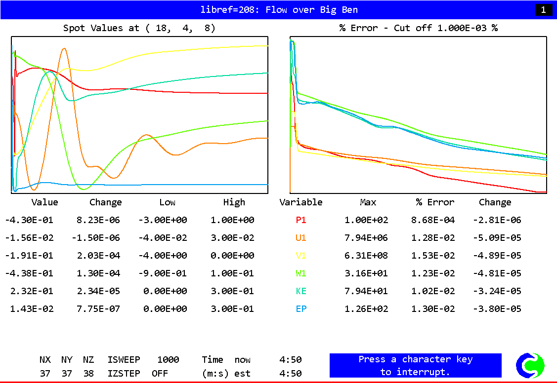
As the Earth solver starts and the flow calculations commence, two graphs should appear on the screen. The left-hand graph shows the variation of solved variables at the monitoring point that was set during the model definition. The right-hand graph shows the variation of errors as the solution progresses.

To the end of the calculation, the monitoring display would be as shown below.

Viewing the results

• Click on the 'Run' button, then on 'Post processor', then 'GUI Post processor (VR Viewer)' in the FLAIR-VR environment.
• When the 'File names' dialog appears, click 'OK' to accept the current result files.
• Click on the 'V' (Select velocity) button, followed by the 'Contour toggle' button, . You will see the velocity contours displaying on Y plane as shown below.

• Click on 'Contour toggle' button to clear the velocity contours.
• Click on 'P', the 'Select pressure' button
• Right click on 'Object management' button, on the control panel.
• Change BLOCKAGE to 'Paint all' on the Hide/Show/Paint dialog box as show below

• Click on 'OK'. The pressure distribution upon the Big Ben will be displayed as shown below

Saving the case

Once a case has been completed, it can be saved to disk as a new Q1 file by 'File - Save working files'. The Q1 and associated output files can be saved more permanently by 'File - Save as a case'.