The workshop is concerned with the prediction of the transient temperature distribution in a metal bar, heated at one end.
The bar is 0.1m long, 0.01m high and 0.005m thick. It is made of steel, and one end is held at a constant temperature of 100 oC. All the other surfaces are assumed to be adiabatic. The initial temperature is 10 oC.
We require the temperature variation of the other end during a period of 10 minutes.
The simulation is two-dimensional and its geometry is shown below.
The geometry and simulation options are set up using VR Editor, the calculations are performed using the PHOENICS solver, EARTH, and the results are viewed using VR Viewer. Only temperature need be simulated.
We will use the X-Y plane for the calculation.
From the system level:
To enter the PHOENICS-VR environment, click on the PHOENICS icon on the desktop, or click on Start, programs, PHOENICS, PHOENICS.
From the commander level:
To enter the PHOENICS-VR environment, click on the 'Run vre' icon in the left column.
In PHOENICS-VR environment,
Start with an 'empty' case - click on 'File' then on 'Start New Case', then on 'Core', then click on 'OK'; to confirm the resetting.
To enter VR Editor:
This is the default mode of operation.
Set the domain size, grid and time steps:
Click on 'Main Menu' and set the title to 'Transient Heat Conduction'
Click on 'Geometry'.
Change the X-Domain Size to 0.1 m.
Change the Y-Domain Size to 0.01 m.
Change the Z-Domain Size to 0.005 m.
Set the number of cells in X to 60.
Set the number of cells in Y to 8.
Leave the number of cells in Z at 1.
Click on 'Steady' to toggle to 'Transient'.
Click on 'Time step settings'.
Set the 'Time at end of last step' to 600s.
Set the 'Last step number' to 120. This will produce time steps of 5s each.
Click 'OK' to close the Time step settings dialog.
Click 'OK' to close the Grid mesh settings dialog.
Activate solution of variables:
Click on 'Models'.
Set 'Solution for velocities and pressure' to OFF
Click on 'energy equation' and select 'Temperature' as energy formulation.
Set the material properties:
Click on 'Properties'
Click on the button next to 'The current domain material is:'. Select 'Solids' from the list of material types, then 'Steel' from the list of solids.
Set the ambient temperature to 10.
Set the solution control parameters:
Click on 'Numerics'
Set the Total number of iterations to 50. This is the number of iterations (sweeps) performed on each time step.
Set the output parameters:
Click on 'Output', then on 'Settings' next to Write flow field.
Set the 'Intermediate field dump' to ON. Leave the step frequency to 1 and leave the 'Start letter' as blank. This will instruct the Earth solver to create a special output file, in which the Z axis is time, and each Z plane is the X-Y solution at that time.
Click on 'Previous panel', 'Top menu' and then on 'OK'.
Click 'Reset' on the Movement control panel, then 'Fit to window' to re-scale the view to fit the geometry.
Use the 'View down' button on the handset to rotate the image so that you are looking at the X-Y plane.
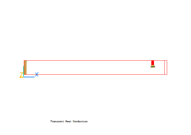
Create the Hot end:
Click on 'Settings', 'New', 'New Object', 'Plate' and select the X plane for the plate to lie in.
Change name to HOT.
Click on 'Size' and set SIZE of object as:
Xsize: 0.0
Ysize: 'To end'
Zsize: 'To end'
Click on 'Place' and set POSITION of object as:
Xpos: 0.0
Ypos: 0.0
Zpos: 0.0
Click on 'General'.
Click on 'Attributes', then on 'Adiabatic'. Select 'Surface temperature' from the list of heat sources. Enter 100 as the Value.
Click on 'OK' to exit the Attributes dialog and on 'OK' to exit the Object specifications Dialogue Box.
Create a temperature probe:
Click on 'Settings', 'New', 'New Object', 'Point_history'.
Change name to PROBE.
Click on 'Size' and Set SIZE of object as:
Xsize: 0.001
Ysize: 0.001
Zsize: 0.005
Click on 'Place' and Set POSITION of object as:
Xpos: 0.09
Ypos: 0.006
Zpos: 0.0
Click on 'General'.
Click on 'OK' to exit from the Object Specifications Dialogue Box.
In the PHOENICS-VR environment, click on 'Run', 'Solver'(Earth), and click on 'OK' to confirm running Earth.
In the PHOENICS-VR environment, click on 'Run', 'Post processor',then GUI Post processor (VR Viewer) Viewer)'. Click 'No' next to 'Use intermediate files' to toggle to 'Yes', then click 'OK' to read the file.
Click on 'Settings', then 'Editor parameters'. Set the Z scale to 0.00008 (remove one zero from the default setting). Set the Snap Size to 0.000001, otherwise the Probe will move too far for each click on the probe position buttons.
Select temperature as the plotting variable, and turn the Contours on.
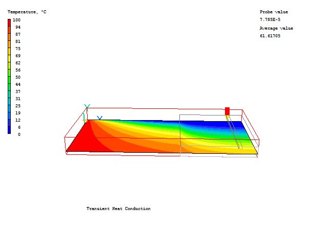
Note that the Z axis now represents time, not distance.
Contours in the Z plane show the temperature distribution at a point in time.
Contours in the Y plane show time variations at particular Y locations as shown below.
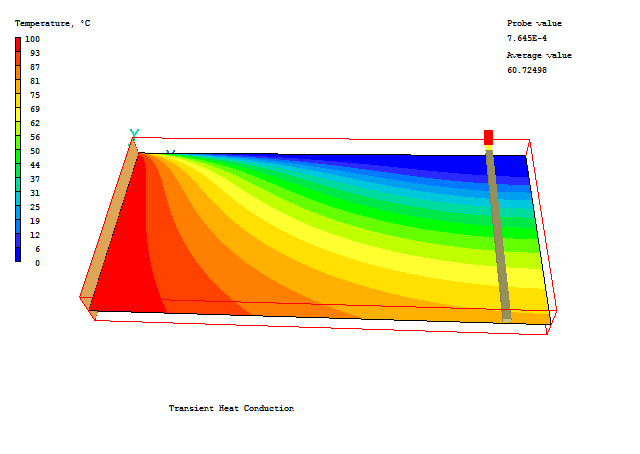
Contours in the X plane show time variations at particular X locations.
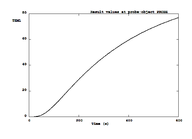
Double-click on the probe object, then click on 'Options' and on the 'Show nett sources' button on the object specifications dialog. The time-history of temperature will be displayed.
In the PHOENICS-VR environment, click on 'Save as a case', make a new folder called 'HOTBAR' (e.g.) and save as 'CASE1' (e.g.).
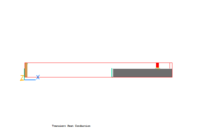
We will now create an insulation object at the far end of the bar.
Click on 'Run - Pre processor - GUI Pre processor (VR-Editor)' to return to the Editor.
Create the insulator:
Click on 'Settings', 'New', 'New Object', 'Blockage'.
Change name to HANDLE.
Click on 'Size' and set SIZE of object as:
Xsize: 0.04
Ysize: 0.006
Zsize: 'to end'
Click on 'Place' and set POSITION of object as:
Xpos: 'At end'
Ypos: 0.0
Zpos: 0.0
Click on 'General'.
Click on 'Attributes', then on 'Other materials'. Select 'Solids', then Epoxy. Click 'OK' to close the Attributes dialog, then 'OK' to close the Object dialog. The geometry is as shown below
In the PHOENICS-VR environment, click on 'Run', 'Solver' then 'Local solver(Earth)', and click on 'OK' to confirm running Earth.
In the PHOENICS-VR environment, click on 'Run', 'Post processor',then GUI Post processor (VR Viewer) Viewer)'. Click 'No' next to 'Use intermediate files' to toggle to 'Yes', then click 'OK' to read the file.
Click on 'Settings', then 'Editor parameters'. Set the Z scale to 0.00008 (remove one zero from the default setting). Set the Snap Size to 0.000001, otherwise the Probe will move too far for each click on the probe position buttons.
Click on the 'Wireframe toggle' button on the hand-set to switch to wire-frame mode. Contours inside the solid will now be visible.
Contours in the Y plane show time variations at particular Y locations - in this case on the lower surface of the bar.
Note that although the temperature stays lower on the lower surface of the insulated region, it is higher on the upper surface of the bar.
In the PHOENICS-VR environment, click on 'Save as a case', and save as 'CASE2' (e.g.). in the folder 'HOTBAR' (e.g.)