- The x-direction is always the angle, q, measured in radians.
- The y-direction is always the radius, r.
- The z-direction is always the axis.
Cartesian and Cylindrical-Polar Co-ordinates
Displaying the Grid
The Default Grid - Auto Meshing
Modifying the GridChanging the Auto-mesh Rules
Changing the Grid Interactively
Manually Changing the Grid by Region
Displaying the BFC Grid
Moving the Probe
Modifying the BFC GridCreating a Grid with the PHOENICS Grid Generator
Importing a Grid Created by an External Grid Generator
Creating a Grid with PIL
Modifying the Grid for an Existing Case
Switching Between Steady and Transient
Setting the Time-Step Distribution Manually
Setting the Time-Step Distribution Automatically
Saving Intermediate Results
Restarting Transient Cases
There are three kinds of spatial grids:
To switch between the co-ordinate systems, click on Menu / Geometry, then on Co-ordinate system. The Cartesian grid is the default.
IMAGE: Grid Mesh Settings Dialog
The change between Cartesian and Cylindrical-polar can be made in either direction.
Note that whilst it is (often) possible to convert existing cases to BFC, it is not possible to reverse the procedure.
Cartesian/Polar cases which cannot be converted are those which use geometries other than cuboids.
Turning the mesh toggle on the hand-set ON by clicking on the Grid mesh ![]() button causes
the current grid to be displayed on the graphics image:
button causes
the current grid to be displayed on the graphics image:
Image: GRID
The grid is displayed on a plane at the probe location. By default the plane is normal to the co-ordinate axis nearest the view direction. For example, if the view direction is along, or close to, +Z, the X-Y plane will be displayed. As the probe is moved or view directions are changed, the grid display will also change to follow.
To manually select the displayed plane, click the pull-down arrow next to the mesh toggle
and choose the required plane. This plane will now be displayed regardless how the view direction is changed, until another direction or 'Auto' is chosen. The position of the plane is still controlled by the probe location.
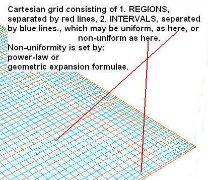
The orange lines shown in the above image are region boundaries. These are automatically created to match the edges of the object bounding boxes (see VR-Editor Object Dialogs - Object Size, Object Positioning), as a consequence of the default ticking of each of the x, y and z options in the 'object affects grid' menu shown below.
If the user removes the ticks, no region is created; nor, of course, are the intervals within them.
This is sometimes desirable; for the user may know that the objects in question, although truly present, can have negligible influence on phenomena of interest. If so, it is time-wasting to allow the grid to be refined around such objects. See Advice on Grid Settings below.As objects are introduced, removed and re sized, the region lines will adapt to match the object layout.
The blue lines are 'ordinary' grid lines. By default, these are distributed by the auto-mesher according to the current set of rules. These are:
Note that if there are no region boundaries in a direction, the auto-meshing will usually assume that only one cell is required in that direction. This is appropriate for 2D cases in which all objects cover the whole domain in the third direction.
If there is an INLET, FAN, OUTLET or PLATE object on the edge of the domain, the auto-meshing will assume that grid is required in that direction, even if there is only one region.
Users should always inspect the grid visually to satisfy themselves that it is appropriate to their purposes. The default auto-mesh settings may sometimes be found to have created a rather coarse grid, suitable for first-exploration runs but not for realistic simulations. It is equally possible that they have created too fine a grid; or one that is fine in the wrong places. 'Object affects grid?' is too important a question for users to disregard.
In most cases auto-set grids will require adjustment, either by changing the auto-grid rules or by manual adjustment before the final runs are made.
Clicking on the mesh with the left mouse button whilst the grid mesh display is on will show the Grid Mesh Settings Dialog. The selected regions will be highlighted in blue, as shown below. The cursor was in the top-right corner of the mesh when the left mouse-button was clicked.
Image: GRID Mesh SETTINGS - Auto
Entering a different region number in the 'Modify region' input box will cause that region to be highlighted instead.
By default, the auto-meshing feature is turned on, as shown in the image above.
The grayed-out values cannot be changed from this dialog unless the auto-mesh is turned off for any direction, as shown here:
Image: GRID Mesh SETTINGS - Manual
Settings on this dialog which are common to auto-mesh on or off are:
Changing the Auto-mesh Rules
When the auto-grid setting is ON or AUTO, the grid in that direction is generated based on certain rules. These are:
When the grid is automatically generated, the normal grid settings in that direction are inactive. To modify one of the regions, the automatic grid must be turned off.
To change the auto-mesh settings for any direction, click 'Edit all regions in' on the Grid Mesh Settings dialog for the direction in question. The following dialog will appear:
Image: X Direction Auto-mesh Settings
The grayed-out values cannot be changed manually unless the auto-meshing is turned off. They reflect the settings generated by the current auto-mesh control parameters.
The 'Reg'(ion) button causes the selected region to be highlighted in in blue in the graphics display. You may have to drag the dialogs to the side to get a clear view of the mesh display.
The following settings influence the auto-meshing:
Version 2017 V2 onwards:
Min cell factor 0.01
Max cell factor 1.0
Max size ratio 1.5
Expansion power 1.1
Expansion form Geometric Progression
Boundaries Auto
Earlier Versions
Min cell factor 0.005
Max cell factor 0.05
Max size ratio 1.5
Expansion power 1.2
Expansion form Geometric Progression
Boundaries Off (On for Flair)
When set to ON, the grid in the first region expands symmetrically from the domain boundary and the first region boundary. This would be appropriate if the domain boundary were a plate or inlet, where changes in flow are expected.
When set to AUTO, the grid expands symmetrically if a PLATE, INLET, FAN, OUTLET or WIND_PROFILE object is detected at the start of the domain. If a WIND object is detected, the grid will expand symmetrically from the ground and side boundaries.
When set to ON, the grid in the last region expands symmetrically from the domain boundary and the start of the last region. This would be appropriate if the domain boundary were a plate or inlet, where changes in flow are expected.
When set to AUTO, the grid expands symmetrically if a PLATE, INLET, FAN, OUTLET or WIND_PROFILE object is detected at the end of the domain. If a WIND object is detected, the grid will expand symmetrically from the ground and side boundaries.
Minimum cell-size ratio.
Maximum cell-size ratio.
These are the ratios between the size of the first cell in a region and the last cell in the previous region, and the last cell in a region and the first cell in the next region. They should both be within the set limits.
Minimum region-boundary cell-size
Maximum region-boundary cell-size
These are the smallest and largest cells at either end of a region. They should both be larger than the set minimum value, unless the region itself is smaller than the limit.
As well as progressively increasing the number of cells in this region, the cells are distributed using a geometric or power-law expansion. To keep the cell distribution with the region uniform the expansion power should be set to 1.0.
The grid is expanded using a symmetrical expansion, except in the first and last regions, where there is choice of symmetrical expansion or expansion from the internal region boundary to the domain edge.
A power of 1 will keep the grid in the region uniform, but may use a lot of cells. Powers > 1 will reduce the number of cells, but will introduce non-uniformity.
Changing the Grid Interactively
Clicking on the mesh with the right mouse button whilst the grid mesh display is on will show the interactive Auto Meshing Dialog.
Moving the slider to the left will reduce the minimum cell fraction or size and hence increase the number of cells in the selected direction. Moving it to the right will increase the minimum cell seize and hence reduce the number of cells. Alternatively, an exact value for the minimum size can be entered into the data input box, and the number of cells will be updated. The box showing the number of cells is display-only. It is not possible to directly enter a specific number of cells.
Manually Changing the Grid by Region
When the auto-meshing for a direction is turned off, the number of cells in any region, and the distribution within any region, can be set by clicking on the region to be modified. The initial region settings will be those created by the auto-mesher. Clicking on X region 3 and Y region 1 of the example shown previously, for example, brings up the dialog box shown below:
Image: GRID Mesh SETTINGS - manual
The diagram below shows a simple three-part grid. Region 1 has 10 cells with a power of -1.5. Region 2 has 10 cells with a symmetric power of 1.5, and region 3 has 10 cells with a power of +1.5.
Image: DIAGRAM 1
The next diagram shows the same grid, but with geometrical expansions in all three regions:
Image: DIAGRAM 2
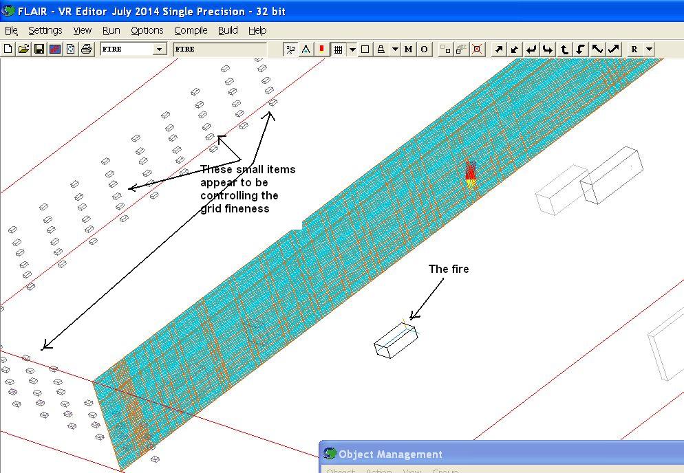
The two most important pieces of advice to the user who has allowed the grid to be created by the automesher are:
An example is shown by the following picture which shows the automeshed grid for the simulation of what happens when a car catches fire in a car park. The car, one might suppose, is of greatest interest, and so should have the finest grid. However automesher has paid attention to the numerous small ventilation apertures in the car-park wall; and, precisely because of their smallness, has created a grid which fits them.
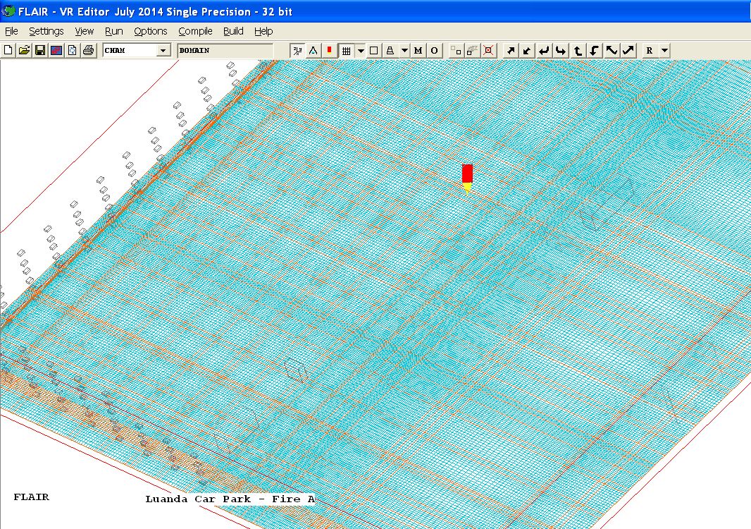
Having recognised that automeshing has created a grid which, because it is very fine, will require large computer times but ignores his needs, what should the user do? The answer depends upon his expertise level.
Many would do best to seek from CHAM, or from their in-house experts, a Q1 file which corresponds better to reality and to their desires. Do-it-yourselfers however, who wish be their own in-house experts, should proceed as follows:
The actions will now be discussed in more detail.
Distinct purposes might be:
Whichever is the purpose, the grid which automesher created is totally unsuitable.
Let us suppose that inquiry shows that whoever commissioned the simulation had purpose (b) in mind, and that the scenario specification consisted of:
If that is the case, it must be admitted that a CFD simulation is not truly needed at all; for a back-of-envelope sum will indicate the ratio of the rates of smoke production and extraction.
However, if CFD is to be used, a 20-by-20-by-20 grid will suffice to demonstrate that the back-of-envelope sum was not far wrong.
How would the extractor devices be represented in such a model? Fixed-mass-flux patches at the walls would be quite good enough.
All BFC library cases, and all user-generated BFC cases can be loaded into PHOENICS-VR.
The possible methods of grid generation are:
Turning the mesh toggle on the hand-set ON by clicking on the Grid mesh ![]() button causes
the current grid to be displayed on the graphics image:
button causes
the current grid to be displayed on the graphics image:
Image: BFC Grid
The grid is displayed on a plane at the probe location. The plane is normal to the co-ordinate axis nearest the view direction. For example, if the view direction is along, or close to, +Z, the X-Y plane will be displayed. As the probe is moved or view directions are changed, the grid display will also change to follow.
In a multi-block grid, the grid will be displayed in the block containing the probe.
In BFC, the probe can only be moved from cell-centre to cell-centre. The probe location is always in IX, IY, IZ.
In a multi-block case, these are shown in 'big' grid co-ordinates, not in local block co-ordinates. Any cell can be moved to directly by typing the cell IX,IY,IZ values into the hand-set.
Note the colouring of the block containing the probe:
In a complex multi-block case, this will help in identifying which way to move the probe.
To move the probe from one block to the next, move up to a linked face, and then step through it by continuing to move in that direction.
The axis colouring will jump to the next block. If the Move probe button is kept pressed, and the IJK orientation of the next block is different, the probe may take off in an unexpected direction - it may even jump back to the previous block if the axes are reversed!
To enter the Grid Generator, turn the grid display ON by clicking on the Grid mesh
![]() button.
Click on the grid anywhere in the domain. The BFC Menu will appear.
button.
Click on the grid anywhere in the domain. The BFC Menu will appear.
IMAGE: BFC Menu
The main functions on the BFC Menu are:
For those users not familiar with the BFC grid generator, several tutorials are available, reached from POLIS / Learn / BFC tutorials. There is also a lecture, reached from POLIS / Learn /Lectures describing... / Body-fitted co-ordinates; introduction describing the fundamentals of BFC Grid generation.
The images above show the geometry created by the BFC tutorials.
Whatever external grid generator is used, the outcome will be a skeleton Q1 called case.Q1, and at least one grid file. If the case is a multi-block case, there will be one grid file for each block.
The skeleton Q1 file will contain a READCO command to read the grid file(s), and instructions for linking the blocks.
An example skeleton file for a single-block grid stored in the grid file grid1 must contain at the very least:
TALK=T; RUN(1,1)
BFC=T
READCO(grid1)
STOP
It may also contain (M)PATCH statements locating boundary conditions, and also COVAL commands setting inlet values.
To import this into PHOENICS-VR, click on File - Open existing case from the top bar of the main VR-Editor/Viewer graphics window. Double-click on case.Q1 to open it in PHOENICS-VR.
Note: The grid files must be in the current working directory, OR the READCO(filename+) command must be modified to include the path to where they are.
Please ensure that the skeleton Q1 is copied to the working directory as case.Q1, together with all the necessary grid files. Use File - Open existing case to open case.Q1.
If the user is familiar with the PIL GSET suite of commands, the Q1 can be edited to create the grid in any convenient way. PHOENICS-VR will recognise and retain all GSET commands.
It does not recognise the older SETPT, DOMAIN, SETLIN or MAGIC commands. If the grid is built with these, or some of these commands are used to smooth parts of the grid, use the DUMPC(name) command to write out a grid file, and supply PHOENICS-VR with a Q1 that just contains:
TALK=T;RUN(1,1)
BFC=T
READCO(name)
STOP
The final result should be a file called case.Q1, which either contains the required GSET commands, or a READCO to read an existing grid file (or files).
Often, once a case has been set up and run, it becomes obvious that the original grid is inadequate. It may be generally too coarse, or grid may be concentrated in the wrong places.
If the grid was generated in the PHOENICS Grid Generator, this can be used to modify the grid as required. On exit from the Grid Generator, most of the objects will have to be re-located and re-sized , as they will still be in their original IJK positions.
If the grid was generated externally, in many cases this can be avoided. Re-enter the grid generator and modify the grid as required. Save the PHOENICS output file with a different name to that used for the original grid.
In VR-Editor, click on Main Menu - Geometry - Read new geometry from file. This will bring up a file browsing window, which will allow the selection of the new Q1 written by the grid generator. The new grid will be read in, and boundary condition locations will be remapped to the new grid when Open is clicked. Note that only boundary conditions common to both grids will be remapped.
To simulate transient behaviour, time is discretised in a similar way to the space dimensions. The Earth solver produces a solution for each step in time before advancing to the next step. An extra term is automatically added to the equations solved, which expresses the influence of the previous time-step.
The default equation formulation is implicit, so there are no extra stability criteria to satisfy when setting the size of the time-steps. If the steps are too large, the details of the transient behaviour will not be picked up.
In Transient mode, objects representing sources will have additional dialogs allowing start and end times to be set.
To switch from Steady to Transient, click on the Steady button on the Grid Mesh Settings dialog,
or in BFC,
on the BFC menu dialog. A new button labeled Time Step Settings will appear.
The Steady button will now be labeled Transient. To switch back to Steady, click on Transient.
Clicking on the Time Steps button displays the Time Step Settings dialog. By default, the time step distribution is set on this dialog before the solution commences.
IMAGE: Manual Time Step Settings dialog
Time can be divided into regions by the Split Regions button. Within each time region, the number of time steps can be set, together with a geometrical or power-law size distribution.
Within each time region, the time step will be the size of the time region divided by the number of steps in that region, allowing for any power-law or geometrical non-uniformity.
When the Automatic Time steps option is turned ON, the time step setting dialog changes to this.
IMAGE: Automatic Time Step Settings dialog
On this dialog, the inputs are as follows:
dt = Courant * minimum cell size / maximum velocity
Apart from step 1, the time step size for each subsequent step is determined by the Earth solver based on the target Courant Number. A table file, dt.csv, is automatically created containing the time step size and cumulative time for each step.
The cumulative time, step size, step number and sweep number are all written to the solution file (phida or phi) so that the Viewer can display the actual cumulative time during a transient animation.
To save intermediate results for plotting in the VR-Viewer or any other post-processor, click on 'Main menu', 'Output', 'Write flow Field'. The following dialog will appear:
IMAGE: Transient Field dumping dialog
Turn Intermediate field dumps to ON
IMAGE: Transient Field dumping dialog
Set the step frequency for dumping. If dumping is not to start at step 1, or finish before the and last time step, the 'Limits' dialog allows the first and last steps to be set. Set a start letter for the intermediate output files. A start letter of A, and a dump frequency of 1 will result in files called A1, A2, A3 etc being dumped at the end of each time step.
The letter Q should not be used, as the file dumped on step 1 will overwrite the Q1 input file!
The size of the intermediate files can be reduced by choosing not to dump each variable to the file. Changing the Y to an N in the 'Dump to file' line will prevent that variable from being written to the intermediate file. If the property-marked variable, PRPS, is so excluded, Viewer will not be able to determine which cells are blocked. Depending on which variables are excluded, it may not be possible to restart the calculation from the intermediate files. All variables are written to the final solution files (PHIDA or PHI and PBCL.DAT) regardless of the dump settings.
If the case is 2D in X and Y, the start letter can be left blank. In this case, a special output file called PARADA or PARPHI is written, in which the results of each time step are saved as a Z plane. In the viewer, sweeping through Z in effect sweeps through time.
To print flow fields to the RESULT file every time step, go to 'Main menu', 'Output', 'Print to Result file', and set 'Step frequency for printing' to 1.
Note that the intermediate output files are optionally saved by 'File', 'Save as a Case', and restored by 'File', 'Open existing case'. The output files can be big and numerous, so it may be better to either ZIP them up, or copy them to a CD for safe-keeping.
The intermediate files can be selected for plotting in the Viewer by choosing 'Use intermediate step files - Yes' on the 'File names' dialog displayed when the Viewer starts.
There are two main possibilities:
To restart and continue the run, bring up the Manual Time step setting dialog, or the Automatic Time step setting dialog.
For manual time step setting, in the 'Time at end of last step' box, enter the new extended end time of the run. Leave 'Time at start of step 1' at zero. In the 'Last step number' box, enter the new total number of steps. In the 'First step number' box, enter the previous last step+1. A dialog will appear asking if a restart is to be activated. Click 'Yes'. The restart will be activated, and the names of the restart files will be deduced from the start letter chosen for saving the intermediate fields.
Please check that the names are correct. To force a restart from the final solution files which are guaranteed to contain all the solved and stored variables, set the 'Solution file' to phida (or phi) and the 'Cut-cell file' to pbcl.dat.
For example, the original run did 100 steps from time 0.0s to 10.0s ( thus giving time steps of 0.1s each). It is now desired to do the next 10.0s with the same time step size. Set 'Time at end of last step' to 20.0, 'Last step number' to 200, and 'First step number' to 101. To activate the restart, click on 'Yes' when asked about activating the restart.
To restart from an intermediate step, say step 50, just set 'First step number' to 51. A dialog will appear asking if a restart is to be activated. Click 'Yes'. The restart will be activated, and the names of the restart files will be deduced from the start letter chosen for saving the intermediate fields.
IMAGE: Time Step Settings dialog for restart
The names of the restart files are also displayed on (and can be set from) the 'Main Menu', 'Initialisation' panel. An active restart is shown by all the initial values (FIINIT) being shown as READFI.
Set the first and last step numbers to the required values. Setting the first step greater than one will trigger the restart. A dialog will appear asking if a restart is to be activated. Click 'Yes'. The restart will be activated, and the names of the restart files will be deduced from the start letter chosen for saving the intermediate fields.
Please check that the names are correct. To force a restart from the final solution files which are guaranteed to contain all the solved and stored variables, set the 'Solution file' to phida (or phi) and the 'Cut-cell file' to pbcl.dat.
The cumulative time at the start of the first step will be read from the specified restart file, and the time step size for the first step will be calculated based on the target Courant Number, maximum velocity and minimum cell size as described above.