VR Viewer Overview
Selecting the Files to Plot
VR-Viewer Environment
VR-Viewer Hand-set and Toolbar Icons
The Main Menu dialog
The Object Dialog Box
VR-Viewer Scripting (Macro) facility
The function of the VRV Macro
Saving MACROs
Running MACROs
MACRO Commands
PHOTON USE Files
Short cuts to Viewer functions:
Short cuts to Viewer Macro commands:
The VR-Viewer is the solution visualisation counterpart of the VR-Editor. It is accessed from Run - Post processor - GUI Post processor (VR Viewer) on the main VR-Editor window. It can display;
Typical plots showing all graphics elements are shown below:
Viewer screen and hand set
Typical line plot
At first glance, the VR Viewer looks very similar to the VR Editor. There are however differences in the controls and graphics-window annotations that facilitate viewing results on the flow domain, for example:
Any combination of colouring modes is allowed.
The streamlines can be animated as balls, vectors or line segments.
Further details of all the hand-set buttons and main window menus are given below.
The files to be plotted are selected during the VR-Viewer start-up sequence. If another set of results is to be plotted, clicking on the F6 icon or pressing the F6 function key will display the file selection dialog without changing any of the display settings. Clicking on 'File' - 'Open existing case' or 'File' - 'Reload working files' will restart the Viewer and reset all the display settings to default.
Steady-State Cases
When the VR-Viewer starts, or when F6 is pressed, it displays this dialog box:
To plot the most recent results, click 'OK' and the VR-Viewer will read the default files and display the first image. If intermediate dumps have been selected, 'Latest dumped files' will display the name of the most-recently written file. If the solver run has finished, the name will be phi (or phida) as shown.
Pressing F9 or clicking the F9 icon will load the most recently-dumped files and refresh the screen image with the new results. This is useful when the Earth solver is still running and is dumping solution files at regular intervals. Pressing F9 will update the screen image using the most-recently written solution files.
A right-click on F9 will cause Viewer to update the screen image automatically each time a new solution file is written by the Earth solver.
The Use intermediate sweep files button is displayed if intermediate dumps have been selected in the VR-Editor Main Menu - Output - Dump Settings panel. When Use intermediate sweep files is selected, the following dialog is displayed:
The > symbol advances to the next stored sweep,>> to the last stored sweep. Similarly, < and << go back to the previous and first stored sweeps. Clicking or pressing F7 or F8 will also load the previous or next sweep files. Clicking or pressing F9 will load the most recent files.
To plot the results of a different case, click on 'No' next to User-set file names to produce this dialog:
Click on 'Select files' to bring up a dialog which allows the selection the files it is desired to plot. These may or may not have any connection to the current case.
This dialog allows the specification all the files the VR-Viewer might want to read - it is only required to specify those, which are to be different from the default. The BFC grid file is only required if a BFC case is to be plotted, the PARSOL file only if a PARSOL case is to be plotted.
If a name of the form 'name.q1' is specified for the input q1 file, the VR-Viewer will assume that it is required to plot the results of that case, and will change the names of the other files in line with the table shown in VR-Editor - File - Save as a case.
Transient Cases
In a transient case, the dialog is slightly different.
The Use intermediate step files button is displayed if intermediate dumps have been selected in the VR-Editor Main Menu - Output - Dump Settings panel. When Use intermediate step files is selected, the following dialog is displayed:
The > symbol advances to the next stored time-step,>> to the last stored time-step. Similarly, < and << go back to the previous and first stored time-steps. Clicking or pressing F7 or F8 will also load the previous or next time-step files. Clicking or pressing F9 will load the most-recently dumped set of results. Right-clicking the F9 icon will cause Viewer to update the screen image each time the Earth solver writes a new solution file.
The VR-Viewer has a reduced set of pull-down menus, as can be seen above. Only the File, Settings, View, Run, Options and Help menus are active.
These work as in the VR-Editor.
This will exit the entire PHOENICS-VR environment, not just VR-Viewer.
Domain Attributes, Probe Location, Add Text, New Clipping plane, New Plotting Surface, New Track Counter, Object Attributes, Find Object, Editor Parameters, Contour Options, Vector Options, Iso-surface Options, Plot Limits, Xcycle settings, Plot variable profile, Near Plane, Rotation speed, Zoom speed, Depth effect, Adjust lighting
The Add Text, Editor Parameters, View Direction, Near plane, Rotation speed, Zoom speed, Depth effect and Adjust lighting dialogs are the same as in the VR-Editor.
This brings up a dialog box in which the probe location and geometry scaling factors can be set. The units used to display the results can be switched between SI (the default), FPS and cgs.
This brings up the probe location dialog. As well as showing the location of the probe in the domain, the dialog also displays the value of the currently selected variable at the probe. Additional pages on the dialog reveal the location of the maximum and minimum values of the current variable in the domain, and allow the probe and/or the view centre to be jumped there.
This creates a new Clipping plane object. A maximum of two clipping plane objects are permitted in the domain.
This creates a new Plot_surf object. Any number of these can be created, and they are managed through the Object management Dialog as all other objects.
This creates a new Track_counter object. Any number of these can be created, and they are managed through the Object management Dialog as all other objects.
This brings up the object dialog box for the currently-selected object. Only the Colour, Go To, Hide, Result and Texture buttons are active. If no object is selected, the Object Management Panel is displayed.
This brings up the Object Management Panel, which shows a list of all objects. The selected object becomes the current object, and is high-lighted in white.
This leads to the VR-Editor Options dialog box.
This leads to the Contour Options page of the Viewer
Options dialog box, shown below for a right-click on the contour button ![]() . The Select
variable
. The Select
variable ![]() button also displays this dialog.
button also displays this dialog.
This leads to the Vector Options page of the Viewer
Options dialog box, shown below for a right-click on the vector button ![]() .
.
This leads to the Iso-Surface Options page of the
Viewer Options dialog box, shown below for a right-click on the iso-surface button ![]() .
.
This leads to the dialog box shown here.
Plot limits sets a volume within which Vectors, Contours and Iso-surfaces are drawn. The limits can be set in physical co-ordinates or as cell numbers. The limits apply to Contours, Vectors and Iso-surfaces. The values are saved for each saved slice.
When entering values in the data-entry boxes, press the tab key to signal the end of data input.
The X, Y and Z radio buttons set the current slice plane (equivalent to the ![]() buttons), and
the slider bar moves the plotting plane in the selected direction.
buttons), and
the slider bar moves the plotting plane in the selected direction.
In those cases which have X Cycle turned on, an additional menu option is activated. This enables the display of the domain to be repeated a number of time. In Cartesian cases, the default is to repeat once, whereas in polar it is to repeat to give 360� coverage. There are also a number of tick boxes on the X Cycle dialog in which the user can select which items are to be repeated on all domains.
This leads to the
Graph Options dialog shown below. This dialog can
also be reached from the  icon on the toolbar.
This leads to the Options tab of the Viewer Options dialog.
These are as in VR-Editor.
This will mirror the domain and all plot elements in either X, Y or Z. It is not possible to mirror in several directions at once. The following image shows the domain mirrored in the Z direction
The VR-Viewer Run menu contains the same options as the VR-Editor, with the exception that in the Pre processor sub-menu, the 'GUI Pre processor (VR-Editor)' is enabled, and in the Post processor sub-menu, the 'GUI Post processor (VR-Viewer)' is inactive.
This is how to return to VR-Editor.
This is as in VR-Editor.
This is as in VR-Editor.
The Viewer toolbar includes the same General, Domain, Object and Movement toolbar icon groups as the Editor. In these, only the Start a new case icon is inactive. In addition, there are four further icon groups.
Slice toolbar, Animate toolbar, Variables toolbar, Function key toolbar

These lead to the Slice Toggle, Slice Direction X/Y/Z, Contour Toggle/Contour Options, Vector Toggle/Vector Options, Iso-surface Toggle/Iso-surface Options, Streamline Management/Stream Options, Graph Options and Slice Management dialogs described below.

These lead to the Macro, Animation Toggle/Animation Options and Record animation dialogs described below.

These lead to the Select Pressure, Select Velocity, Select Temperature and Select a Variable dialogs described below.
The F3-F5 icons are used to control the VR-Viewer macros.
F6 - F8 control the plotting files, as described above.
F9 loads the most-recently written set of results, preserving the current view and display settings. A right-click on F9 activates the auto file update mode. Each time the Earth solver writes a new solution file, Viewer will read the new file and update the screen image.
The tool bar also displays the name and type of any selected object. If no object is selected, it will display the name of the domain (usually CHAM).
The status bar displays information regarding the progress of the current plot. When reading files, it shows the percentage of the file that has been read. The current working directory is displayed in the status bar when it is not showing other information.
The VR-Viewer hand-set is shown below:
The top two rows of buttons, Axis toggle through to Bounding Box toggle, are exactly the same as in the VR-Editor, except for the Macro and Record animation buttons, which are described in detail later.
The movement controls are also the same as in the VR-Editor, including Fly-through Mode.
The remaining hand-set buttons are described here.
Object Management, Contour Toggle/Contour Options, Vector Toggle/Vector Options, Iso-surface Toggle/Iso-surface Options, Streamline Management/Stream Options, Streamlines from GENTRA Tracks, Slice Toggle, Slice Management, Animation Toggle/Animation Options, Slice Direction X/Y/Z, Select Pressure, Select Velocity, Select Temperature, Select a Variable, Probe position hand-set controls, Show Probe Location, Display Minimum and Maximum Values, Viewer Options 'Options' Dialog, Plot Variable Profile
The object management panel has similar functionality as in the VR-Editor, although the options which allowed the objects to be modified have been disabled. This includes the facility to create or delete objects. There are four additional items on the Action and Context menus. These are:
- draw surface contours,
- dump surface values,
- dump object profile, and
- show nett sources (sums of sources) for selected objects.
These are described in VR-Viewer Object context menu
A left-click turns the display of contours on and off. The display plane is selected by the Slice Direction buttons. The variable used to colour the contours is selected with the Select pressure / temperature / velocity / variable buttons.
The area-averaged contour value for the current plotting plane is displayed under the probe value. The average is taken over the current plotting limits.
A right-click brings up the Contour Options page of the Viewer Options dialog. This dialog can be left open. Any changes made are implemented in the image immediately. The same dialog is opened from Settings - Contour Options or from the Select Variable button. When entering values in the data-entry boxes, press the tab key to signal end of input.
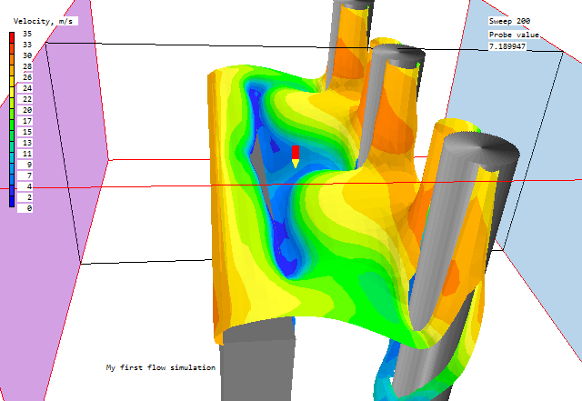
Contours with linear scale
Contours with log10 scale
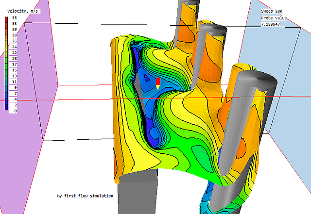
Contours as lines
Filled contours with lines
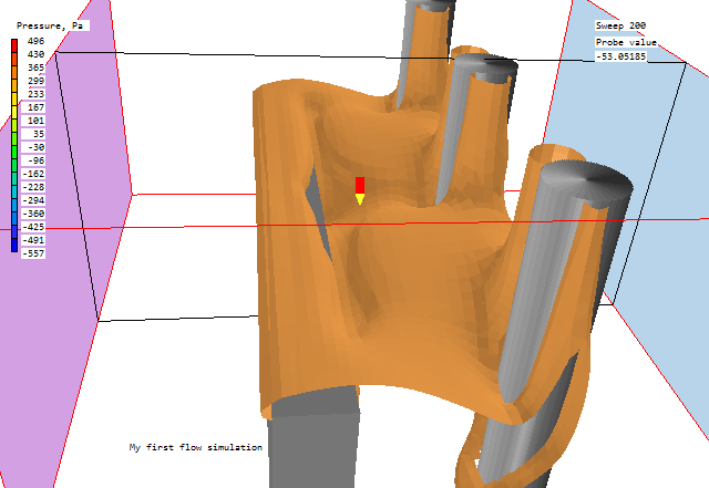
Contour with full pressure range
Transparent contour with reduced pressure range
Filled contour with reduced pressure range
Smoothly shaded contours
Contours with Averaging turned off
If the contours do not change dramatically when switching between averaging on and off, it is an indication that the grid is reasonable. If they do change dramatically, the grid is almost certainly not fine enough to resolve the details of the flow.
Contour labeling
Contours with Automatic Labeling
Contour formatting
The individual colours can then be further adjusted by clicking on the colour sample and using the colour-chooser dialog to fine-tune the colour. The modified palette can be saved to an ASCII text file, or a previously-saved palette can be loaded. Saved palettes can be loaded from Macros.
Contour drawn in Greyscale
A left-click turns the display of vectors on and off. The display plane is selected by the Slice Direction buttons. The variable used to colour the vectors is selected with the Select pressure / temperature / velocity / variable buttons.
A right-click brings up the Vector Options page of the Viewer Options dialog. This dialog can be left open. Any changes made are implemented in the image immediately. The same dialog is opened from Settings - Vector options.
When entering values in the data-entry boxes, press the tab key to signal end of input.
Unlimited vectors
Limited vectors for same case
In IPSA cases, this option has a further effect. When ticked, the vector is multiplied by the volume fraction of the currently-selected phase. This has the effect of removing vectors from regions where the current phase is absent.
This can be used to bring out secondary flow features which are often masked by the dominant flow direction which is much stronger.
The Select Velocity ![]() button will
select Phase 1 or Phase 2 velocity or Vector magnitude according to the vector phase
setting. Similarly, the Select Temperature
button will
select Phase 1 or Phase 2 velocity or Vector magnitude according to the vector phase
setting. Similarly, the Select Temperature ![]() button will select
Phase 1 or Phase 2 temperature.
button will select
Phase 1 or Phase 2 temperature.
Line arrows with line width 3
3D vectors with line width 3
A left-click turns the display of iso-surfaces on and off. The variable used to colour the display is selected with the Select pressure / temperature / velocity / variable buttons. The iso-surface value is usually the value of the selected variable at the probe location. An exact value for the iso-surface can also be set from the Iso-surface options dialog box.
An iso-surface will be drawn for each stored slice, at the value of the current variable at the location the probe was when the slice was stored. This becomes especially apparent in a BFC multi-block case, when several slices may be stored to build up a larger image.
If the iso-surface value is changed from 'probe value' to 'User set', only a single surface will be drawn at the set value.
A right-click brings up the Iso-surface Options page of the Viewer Options dialog. This dialog can be left open. Any changes made are implemented in the image immediately. The same dialog is opened from Settings - Iso-surface options.
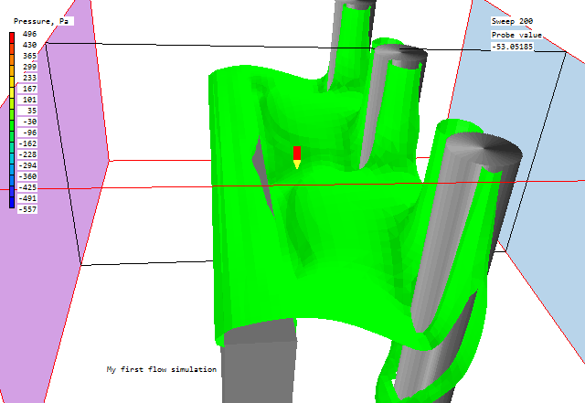
Iso-surface of pressure coloured by pressure
When set to 'Secondary variable', the iso-surface is coloured with a contour map of the selected secondary variable.
Iso-surface of pressure coloured by velocity
The 'Contour appearance' settings on the Contour options panel also apply to the iso-surface contour map.
Fill-and-lines Iso-surface of pressure coloured by velocity
When set to 'Fixed colour', the iso-surface has a uniform colour selected from a colour-selection dialog.
Iso-surface of pressure coloured by user-set colour
Control over the generation of streamlines is exercised through the Streamline Management Panel, shown below.
It is a listbox similar to the Object Management Panel although the contents of the columns are different. From the left they are index, type, X, Y, Z location for the origin of the streamline and visibility flag.
The Streamline Management Panel has three menus Object, Action and Animate which are described below.
Menu item New will generate streamlines according to the Options currently selected.
The second Menu item Options will bring up a dialog where various options for streamline generation may be selected. This dialog also appears when the streamline icon is clicked and no streamlines have been created yet.
The options on this dialog are:
Start along a line
Start around a circle
The line mode for each streamline is stored individually. Changing the 'Coloured by' mode or the Flight time limits will only change the way new streamlines are drawn.
Select All will highlight all the streamlines for subsequent action.
Refresh will repopulate the listbox and clear any current selections.
Close closes the management panel.
The line mode for each streamline is stored. Changing the 'width', 'Flight time' or 'Coloured by' mode will change the way all existing streamlines are drawn.
Actions will apply to all currently selected streamlines. When creating streamlines or groups of streamlines, there are occasions when not all are desired in the final plot. The first three actions therefore give the ability to turn individual streamline visibility on or off or to delete the streamline altogether.
The Streamline location item brings up a dialog which enables the starting location for individual streamlines to be modified.
The last three menu items enable the streamline type, direction and colour to be changed.
Once generated, the streamlines can be animated to give a better impression of the flow pattern. The default animation display (balls radio button active) is to send a single grey sphere along the length of each streamline. The length of the animation will be 100 frames and will repeat until the animation is terminated. The animation control dialog is shown here:
Increasing the number of frames makes the animation smoother, but will slow down the refresh rate. Increasing the number of balls per streamline gives a clearer impression of the path, but also slows the animation down. The best result is a compromise between the number of frames and the number of balls for the particular graphics card in question.
When the Show streamline checkbox is unticked, only the balls (or vectors) will be drawn.
The streamline balls are usually grey. When the Colour by value checkbox is ticked, they will be coloured in the same way as the streamline itself. The size of the balls is controlled by the 'Animation ball size' input box.
When the vector radio button is active, the balls are replaced by moving vectors, which show the local flow direction and speed. The 'Animation ball size' input box is replaced by 'Vector scale'. Vectors look best with the streamline display turned off.
When the line segments radio button is active, the balls are replaced by line segments denoting a set time period. The default time period is 10% of the total flight time. The 'Animation ball size' input box is replaced by 'Segment length'.
The Save button opens a dialog from which an animated GIF file or an AVI of the animation can be saved. The file will contain all the frames chosen for the animation - these can be a sub-set of the frames making up the full animation. For example 1000 frames may be needed for smooth movement, but only 100 frames need be saved to AVI, making a movie lasting 10 seconds at the default 10 frames per second.
GENTRA particle tracks can be displayed as streamlines in the VR-Viewer. The track
information is written to a particle history file called, by default, ghis. To display the
tracks, click the ![]() Streamline button. There will
be a new button at the bottom of the dialog, labeled 'Load GENTRA Track file'. Clicking this
brings up a file browser window to select the file containing the GENTRA tracks. Once selected,
clicking 'Create Streamlines' will display the tracks from the file.
Streamline button. There will
be a new button at the bottom of the dialog, labeled 'Load GENTRA Track file'. Clicking this
brings up a file browser window to select the file containing the GENTRA tracks. Once selected,
clicking 'Create Streamlines' will display the tracks from the file.
Alternatively, click the Macro button on the handset, and enter the name of the history file as the name of the 'RUN macro' file. Click OK to close the Macro functions dialog.
All the track information in the file will be read, and a streamline will be generated for each track in the file. If only selected tracks are required, create a file with any convenient name, and insert into it the lines:
history read
ghis m [n]
where ghis is the name of the history file, m is the number of the (first) track to read, and n, if present, is the number of the last track to read. The file can contain any number of such pairs of lines. This file can now be used as a VR-Viewer macro file.
The new streamlines will appear in the Streamline management panel, and can be operated on as normal streamlines, except that the start locations cannot be changed.
Note: in a transient case, particle tracks will only be displayed for the time steps which fall within their flight time.
This button toggles the display of the saved slices on and off. It is not possible to store slices or delete slices when the slice toggle is off.
The Slice Management Panel offers a limited subset of facilities described for the Streamline Management Panel described above (it has no Options or Animation items).
This makes a copy of the contours and vectors on the slice plane. When the slice plane is moved, the copied image will remain until deleted.
In this way, it is possible to build up a composite image with many planes. The saved slices have an orange border to differentiate them from the current slice, which has a white (or black) border. The image below shows two X slices, a Y slice and a Z slice.
The contour and vector display in the saved slices always follows that of the current slice.
A left-click will cause the Viewer to re-create the current image from each of the saved intermediate files, if any are available. The frequency with which intermediate files are saved by the solver is set from the Output - Dump Settings panel of the Main Menu.
A right-click on the Animation Toggle brings up a dialog from which the animation can be controlled.
The dialog controls the first and last sweeps or steps to be plotted, and the sweep or step frequency of plotting.
Save animation: saves an animated GIF or AVI of the animation. The file name and type will be prompted for each time the animation button is pressed.
Threaded animation: provides user with the option of using a separate thread for
reading the intermediate step PHI files. This is particularly useful when creating animations
from large models as it enables the main window to remain more responsive.
Threaded transient animation is set on by default in the CHAM.INI file.
Save animation as MACRO: opens the MACRO dialog in order to save the current screen set-up as a macro file. The saved macro will end with the 'ANIMATE' keyword.
Units for time display: allows the choice of seconds, milliseconds, minutes, hours or days for the time shown in the top-right corner of the screen.
Once an animation is started, it can be stopped or paused by clicking the appropriate button on the 'Animation progress' dialog which appears.
A paused animation can be continued by clicking 'Continue'.
Clicking the animation button again while an animation is running will stop the current animation, with no possibility of continuing it.
This selects the plane to be used for displaying contours and vectors. The plane always passes through the probe location, so moving the probe moves the plotting plane. This plane is also used when starting streamlines around a circle.
In BFC, these buttons refer to the I, J and K grid co-ordinate directions, and not to the Cartesian space directions. As the probe moves by one cell at a time, the slice also moves by a cell at a time.
In a multi-block case, the contours and vectors are drawn for the block that contains the probe. If plots are required from more than one block at a time, use the Slice Management button to store the current slice, then move the probe to the next block, create another slice, and so on until the entire picture has been built up.
This selects the pressure variable, P1, as the current display variable. It will be used to colour contours, vectors, streamlines and iso-surfaces.
This selects the absolute velocity as the current display variable. It will be used to colour contours, vectors, streamlines and iso-surfaces. For two-phase cases, the velocity will be that of the current vector phase.
This selects the temperature variable, TEM1 (or TMP1 if it is stored), as the current display variable. It will be used to colour contours, vectors, streamlines and iso-surfaces. For two-phase cases, the temperature will be that of the current vector phase.
This brings up the Contour Options page of the Viewer Options dialog box. Any variable can be selected as the current display variable.
These
down/up buttons ![]() move the probe in the X, Y and Z directions. The distance moved each time a
button is pressed is controlled by the Snap size set in the Editor
Parameters dialog box. The bigger the snap size, the faster the probe moves.
move the probe in the X, Y and Z directions. The distance moved each time a
button is pressed is controlled by the Snap size set in the Editor
Parameters dialog box. The bigger the snap size, the faster the probe moves.
In BFC, the probe can only be moved from cell-centre to cell-centre. The probe location is always in IX, IY, IZ.
It is possible to double-click on the data-entry box next to the buttons and type in an exact position. The new position is read when another data-entry box is selected.
To see which cell the probe is in, right click on the Axis Toggle /View Options button ![]() and turn 'Cell
posn' on. The probe cell location will be displayed in the bottom-right corner of the
graphics screen.
and turn 'Cell
posn' on. The probe cell location will be displayed in the bottom-right corner of the
graphics screen.
The probe is also
a pickable item. Double clicking on the probe or clicking the ![]() icon on the toolbar
causes the following dialog to appear:
icon on the toolbar
causes the following dialog to appear:
It contains a quick summary of the data at the current probe location. The current variable can be changed by choosing from the pull down list. The probe location can be moved through the model, either in physical space (X,Y,Z position), or by cell location. When moving in physical space, the Cell location boxes will show the cell centre nearest to the probe. When moving by Cell location, the X,Y,Z boxes will show the physical location of the probe. The 'Set view centre' button centres the view on the probe. The 'Appearance' buttons switch the probe between the default 'pencil' and a sphere. When displayed as a sphere, the colour and diameter can be set from here.
The other pages of the above dialog show the low and high spots for the current variable. If the 'Reveal' checkbox is ticked then the Low and High Spots will be revealed as blue and red spheres respectively. These indicate the position of the minimum and maximum values respectively of the current plotting variable. The 'Set view centre' button centres the view on the Low or High spot, and the 'Move probe here' button moves the probe to the position of the High or Low Spot, bringing with it the contours or vectors if they are displayed,

In order to control the size of the spheres open the Viewer options dialog by clicking
on the 'Select variable' ![]() icon then moving to the final page 'Options'.
icon then moving to the final page 'Options'.
This
dialog is reached by clicking the 'Select variable' icon ![]() , or from
'Settings', 'Contour options' then selecting the Options tab.
, or from
'Settings', 'Contour options' then selecting the Options tab.
This page contains options to:
 );
); 
Clicking on
the ![]() icon
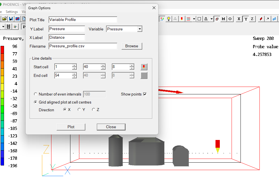
leads to the Graph Options dialog:
icon
leads to the Graph Options dialog:
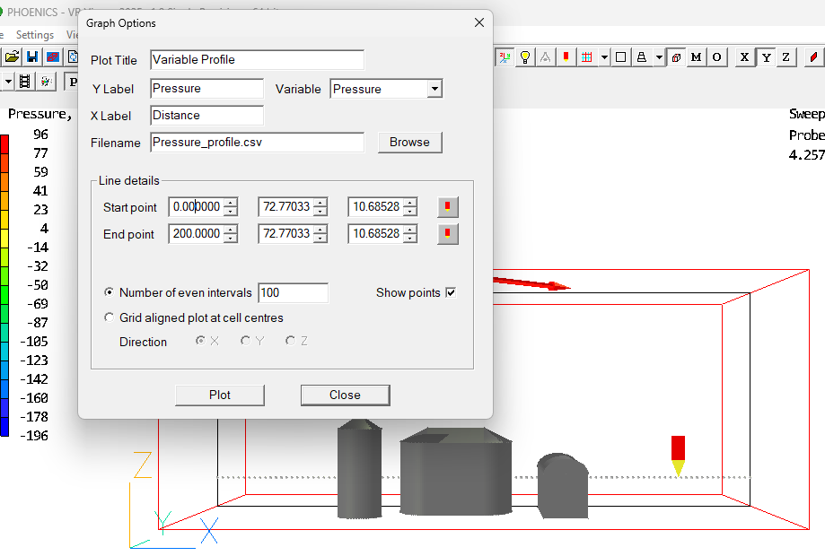
The aim is to create a line plot of a selected variable along a straight line between
two points. The variable to plot is first chosen from the pull down selection; this may be
any of the saved variables in the PHI file. Next the start and end point for the line
should be selected. By default these will be the low and high spot for the current
plotting plane. The ![]() icon will reset the start or end point to the current probe location. The
number of intervals used for the profile is restricted to between 2 and 5000. The
"Show points" check box toggles the display of the profile points in the main
VR-Viewer window, as shown above.
icon will reset the start or end point to the current probe location. The
number of intervals used for the profile is restricted to between 2 and 5000. The
"Show points" check box toggles the display of the profile points in the main
VR-Viewer window, as shown above.
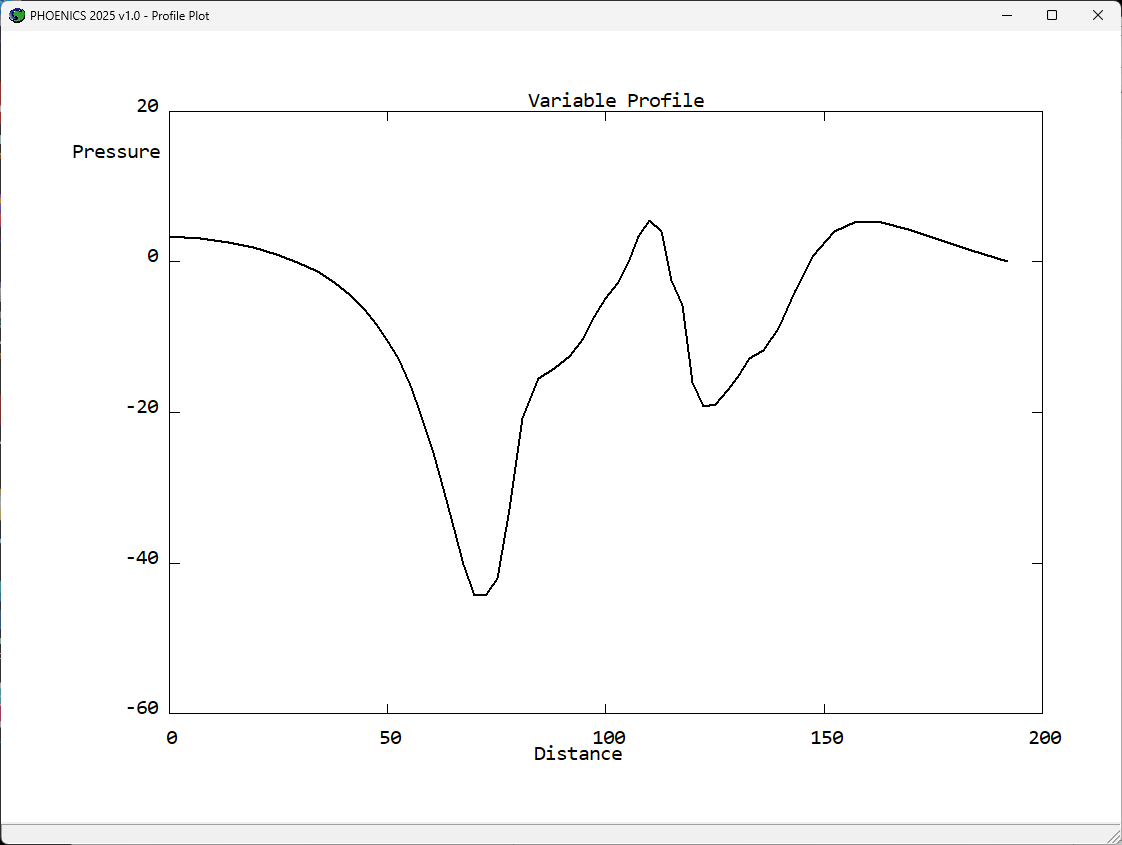
The probe will be moved along the line joining the start and end points, and the value of the selected variable will be saved at the set number of intervals. If contour averaging is turned on, the data will be taken from the averaged field. If it is turned off, it will be taken from the 'raw' data, and sharp steps may be seen at cell boundaries.
Distance is measured along the line, with zero denoting the start point.
The 'Plot' button will display the data as a graph, using the Title and X and Y axis labels from the dialog.
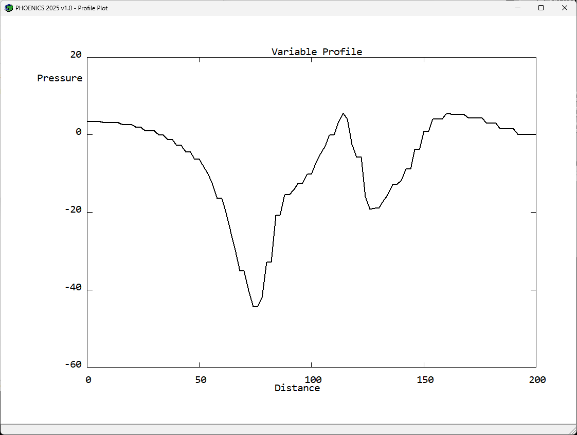
To close the plot, use the left mouse button to click on this window. A hard copy of the profile plot may be obtained using the " Save window as..." option from the File menu. The print option for a profile plot is not currently available.
The data points are automatically saved to the file specified in the 'Filename' input box. By default it is <varname>_profile.csv where <varname> is the name of the selected variable. This file can be easily imported to Excel. It is also compatible with AUTOPLOT.
The appearance of the above line plot is somewhat jagged, this can be improved by reducing the number of intervals to be similar to the number of cells along the plot line. If the plot line is in plane (grid aligned), then one can use the new option to plot at cell centres.
The Main Menu in the Viewer is much simpler than in the Editor.

Note that it is only the contour scale, probe value and average value which are changed - the data is left untouched. The probe location is also shown in the selected unit set.
Just as in the VR-Editor, double-clicking on an object will display the object dialog box.
Unlike in the VR-Editor, the values in the size and position boxes cannot be changed - they display the size and position of the current object. Similarly, the Geometry button on the Shape page is inactive, although textures can still be modified.
The Go To and Hide buttons work as in the VR-Editor. The Colour button allows the colour and/or transparency of an object to be temporarily changed. Permanent changes can only be made in the VR-Editor, and become permanent when the working files are saved.
The Show nett sources button on the Options page has several functions, depending on the object selected. The possibilities are:
When the display window is closed, the contents are automatically written to a text file in the local working directory. The name of the file is the same as the title of the display dialog, with a '.txt' extension.
If 'Show nett sources' is selected for the Domain in the Object Management Dialog, all the sources for all objects, and all force and moment information, will be displayed in the dialog, and subsequently saved to the local text file.
This data is also saved to the same file as the sums of sources.
'Show nett sources' can also be found on the Object Management Dialog action menu, and on the right-click context menu.
To colour an object by the current plotting variable, select the object, right-click on it and select 'Surface contour' from the context menu.
Alternatively select the object or objects from the Object Management Dialog, and then select 'Surface contours' from the Action Menu.
To plot contours or vectors on an arbitrary surface, create a Plotting Surface object. This can be done in the Viewer (or Editor) from 'Settings - New Object - Plotting surface', or from the Object management Dialog, 'Object, New, Plotting Surface'. Double-click the new object to open its Specification dialog, set any desired shape and place it where required.
In the Viewer, select the new object, right-click and select 'Surface contours'.
Now select 'Surface vectors'
When an object is selected, the right mouse button will bring up a context menu for the current object. Most options which allow for the modification of an object have been disabled, except 'Modify Colour'. However, there are five items which are only available in the viewer
In addition, the area-weighted average values of the current plotting variable in the X, Y and Z directions will be displayed in a display dialog, and written to the bottom of the surface_value file. A typical display is shown below:
Both .csv files can be easily imported into Excel for further processing. They are also compatible with AUTOPLOT.
A typical use of a VRV macro is to record a particular view and magnification, and then restore it whenever required, for example when preparing images for a report. Using a macro in this way will guarantee that a sequence of images from different phi files, perhaps generated on separate occasions, can all use the identical view and magnification settings.
A macro file can contain a single image, or a sequence of images separated by PAUSE commands.
Macro command files are ASCII text files, and can be edited (or created) using any convenient text-file editor.
Macro files can be created by the following means:
Select 'Save as new - Yes', enter a filename then click OK. The current view settings will be written to the selected file.
The default filename is vrvlog.
When the setting 'Full or partial' is set to Full, all settings will be written for each frame. This gives a long macro file, but guarantees that the views will be reproduced exactly regardless of the starting condition.
When the setting 'Full or partial' is set to Partial, only non-default settings will be written for the first frame. For subsequent frames, only settings which have changed from the previous fame will be written. This results in a much shorter macro file, but the final effect may depend on the state of the Viewer (view direction, object visibility etc) when the macro is run.
The macro commands can be copied into the Q1 input file, by placing them between the statements VRV USE and ENDUSE. These two lines, and all the macro lines, must start in column 3 or more to ensure that they are treated as comments by the VR-Editor.
Macros can be run by as follows:
The default file name is Q1.
The commands set the state of the VR-Viewer settings. The screen image is updated when a PAUSE command is encountered, or the end of the file is reached. The image is the outcome of the final states of all the settings.
The commands making up the macro language can be divided into a number of groups. Only those commands that change a default or change an existing setting need be placed in the macro file.
The individual commands can be shortened, as long as the remaining part is unique.
Short cuts to commands
| FILE name [xyz name for BFC case] | Sets the name of the PHI (and XYZ file) to plot |
| FILE + | Read the next saved PHI file (equivalent to F8) |
| FILE - | Read the previous saved PHI file (equivalent to F7) |
| USE file | Read commands from another file. Use files can be nested to a depth of 5. |
| VIEW x, y, x | Sets the View direction |
| UP x, y, z | Sets the Up direction |
| VIEW CENTRE x, y, z | Sets the Cartesian co-ordinates of the view centre - the point about which the image rotates. |
| [VIEW DEPTH depth | For the Windows Viewer, sets the View Depth. The default is 3.0. A value of 100000 makes the view isometric] |
| [VIEW TILT angle | For the DOS/Unix Viewer, sets the perspective angle. The default is 0.8. A value of 0.0 makes the view isometric] |
| SCALE scalex, scaley, scalez | Sets the overall domain scaling factors |
| NEARPLANE depth | Sets the near plane position. |
The View Centre, Scale factors and View Depth/Tilt settings can be seen by clicking on 'Reset'.
The primary keyword POSITION is followed by a secondary keyword to identify which item is under consideration. The two integers represent the normalised location in the range 0.0 - 1.0 for the first character of the item. [The origin is at the top left hand corner of the client area.] Each item also has an associated ON / OFF switch to indicate whether it is to be drawn or not.
| POSITION CELL x, y | Shows the current probe position in terms of cells |
| CELPOS ON / OFF | Shows or hides the display of the probe position |
| POSITION CONTOURKEY x, y | Positions the contour colour scale |
| CONTOUR SCALE ON / OFF | Shows or hides the display of the contour key |
| POSITION TITLE x, y | Positions the run title |
| TEXT ON / OFF | Shows or hides the display of the run title |
| POSITION PROBE x, y | Positions the echo of the probe value |
| PROBE ON / OFF | Shows or hides the probe |
| POSITION AXIS x,y | Positions the location of the axes |
| AXIS ON / OFF | Shows or hides the axes |
| AXIS LINE WIDTH ipixel | Sets the axes line width to ipixel |
| AXIS LINE COLOURS icolX, icolY, icolZ | Sets the colours of the X, Y and Z axes to icolX, icolY and icolZ |
Labeling the Plot
| TEXT CLEAR | Deletes all previous text items |
| TEXT size, colour | Sets size (1=large, 4=small) and colour, immediately followed by |
| string | Sets the actual text to be placed on the plot |
| Xpos Ypos | Sets the normalised position of the first character as above |
| VARIABLE name | Sets the name of the current plotting variable |
| VARIABLE RANGE min max | Sets the minimum and maximum values for the plot. |
If the minimum/maximum values are changed from the default (i.e. the current field values), the set values will be used for all subsequent plots for this variable. Setting specific minimum and maximum values ensures that contour plots from different PHI files are scaled consistently.
Contours
| CONTOUR ON / OFF / CLEAR | Clear also deletes all saved slices. |
| CONTOUR FILL ON / OFF | Controls the display of the filled contour bands. |
| CONTOUR LINE ON / OFF | Controls the display of the contour lines between bands. |
| CONTOUR LINE COLOUR index / MULTI | Controls the colour index of the contour lines between bands. MULTI indicates using contour band colours. |
| CONTOUR LINE WIDTH ncwid | Controls the width in pixels of the contour lines between bands. |
| CONTOUR SCALE ON / OFF | Controls the display of the contour scale. |
| CONTOUR OPAQUENESS iopaq | Sets the contour opaqueness to iopaq. |
| CONTOUR BLANK ON / OFF | Sets the out-of-range transparency. |
| CONTOUR AVERAGE ON / OFF | Sets contour averaging on or off. |
| CONTOUR CONTINUOUS ON / OFF | Sets the contours to use smooth shading |
| CONTOUR INVERSE ON / OFF | Inverts the colour scale so that red is low and blue is high |
| CONTOUR GREYSCALE ON / OFF | Switches the contour colours to greyscale. Note that this will also affect vectors and iso-surfaces. |
| CONTOUR RANGE Vmin Vmax [LOG] | Sets the contour range to be Vmin to Vmax. The optional last argument LOG switches to a log10 scale. |
| VECTOR ON / OFF / CLEAR | Clear also deletes all saved slices. |
| VECTOR SCALE vscal | Sets the vector scaling factor |
| VECTOR REFERENCE vref | Sets the vector reference velocity |
| VECTOR INTERVALS intx, inty, intz | Sets the vector plotting frequency |
| VECTOR PHASE 1 / 2 | Sets the phase for the vectors |
| VECTOR COLOUR n | Sets the vector colour to colour number n |
| VECTOR WIDTH ipixel | Sets the vector width to ipixel pixels |
| VECTOR TYPE type | Sets the vector type to TOTAL or IN-PLANE |
| VECTOR MAXLENGTH maxlen | Sets the maximum vector length (m/s) |
| VECTOR COMPONENTS var1, var2, var3 | Sets the names of the vector component variables. |
If the vector scale or reference is changed from the default, this value will be used for all subsequent vector plots. Setting a specific vector reference will ensure that vectors from different PHI files are scaled consistently.
| SURFACE ON / OFF | |
| SURFACE VALUE surfval | Sets the surface value, otherwise uses the probe value if not set. |
| SURFACE COLOUR iPalette | Sets a colour from the VR palette to colour the surface by, otherwise uses the contour colour associated with surface value. |
| SURFACE COLOUR iRed iGreen iBlue | As an alternative to setting palette index one may set RGB values (0-255) to colour the surface by. |
| SURFACE VARIABLE variable | Sets a secondary variable the surface contour will be coloured by. The VARIABLE RANGE (for contours) will now apply to this secondary variable. |
| SURFACE VARIABLE OFF | Turns off any secondary variable the surface contour will be coloured by. |
| SURFACE OPAQUENESS iopaq | Sets the surface opaqueness to iopaq, unless a secondary variable indicated in which case the CONTOUR OPAQUENESS setting is used. |
| STREAM DELETE / CLEAR | Clear also deletes all saved slices. |
| STREAM x y z | Start a streamline at (x,y,z) |
| STREAM MODE line/arrow/ribbon | Set stream mode |
| STREAM DIRECTION downstream/upstream/both | Set stream direction |
| STREAM COLOUR variable/track/total | Set stream colour mode |
| STREAM ORIGIN probe/line/circle | Set stream start point |
| STREAM START x y z | Set start of line for start along line |
| STREAM END x y z | Set end of line for start along line |
| STREAM RADIUS rad | Set radius for start around circle |
| STREAM TIME tmin tmax | Set minimum and maximum track flight time |
| STREAM TRACKS ntrack | Set number of tracks for line or circle mode |
| STREAM WIDTH ipixel | Set the streamline width to ipixel |
| STREAM DRAW | Create streamlines based on current mode settings |
A secondary keyword, ANIM, is added to streamlines. By default the animation will be with a grey ball. Optional keyword COLOURED for animation balls to be coloured appropriately. Alternatively VECTOR will produce coloured vectors.
| STREAM ANIM BALL [COLOURED] | Animate as balls |
| STREAM ANIM VECTOR | Animate as vectors |
| STREAM ANIM SEGMENT seg_length | Animate as segments with length seg_length |
The secondary keyword FREQUENCY has two integers, the first is the number of frames per cycle, the latter the number of balls or vectors .
| STREAM FREQUENCY nframe nball | Set number of frames and number of balls or vectors. |
| STREAM VISIBILITY [ON/OFF] | Determines the streamline visibility during animation. |
The ball size and vector scale are set as shown below.
Although the keyword CONTOUR is used to control this feature, the same palette is used for all plotting elements - contours, vectors, iso-surfaces and streamlines.
CONTOUR NUMCOLS numcols sets the number of colours used to numcols. If the line is absent, the current number of colours will be used.
CONTOUR PALETTE iRed, iGreen, iBlue sets the red, green and blue values. Values are in the range 0 - 255. There must be numcols lines, one to define each colour. If these lines are absent, the current palette will be used.
If the number of colours is set to 4, the colours will red (255 0 0), yellow (255 255 0), green (0 255 0) and blue (0 0 255).
As an alternative, the name of a palette file can be specified by using:
CONTOUR PALETTE filename where filename is the name of the palette file. A palette file can be saved from the 'Update palette' option of the Contour Options dialog. The format of the file matches the 'CONTOUR NUMCOLS','CONTOUR iRed, iGreen,iBlue' format described above. The default 16-colour palette is given here:
VR Contour palette
16
255 0 0
255 66 0
255 128 0
255 176 0
255 224 0
255 255 48
192 255 0
100 255 0
0 255 0
0 232 72
0 220 160
0 200 220
0 160 240
0 120 255
40 40 255
0 0 255
| LINE START x,y,x | Sets the start point of the line |
| LINE END x,y,z | Sets the end point of the line |
| LINE NPOINTS np | Sets the number of points to extract along the line |
| LINE XLABEL label | Sets a label for the X axis (must be only item on line) |
| LINE YLABEL label | Sets a label for the Y axis (must be only item on line) |
| LINE TITLE title | Sets a title for the plot (must be only item on line) |
| LINE DUMP SIZE nx,ny | Sets the size in pixels of the saved image file |
| LINE DUMP file_name | Sets the name of the GIF file of the time plot. To save pcx, bmp or jpg add the required extension (must be only item on line) |
| LINE FILE file_name | Sets the name of the saved data file (must be only item on line) |
| LINE PLOT | Creates the plot and saves files using latest settings |
The variable plotted is the current plotting variable, set with VARIABLE name, as above.
| TIMEPLOT OBJECT name | Sets the name of the POINT_HISTORY object to take data from |
| TIMEPLOT VARIABLE name | Sets the name of the variable to be plotted. It must be one of the variables selected for storage at the named POINT_HISTORY object. |
| TIMEPLOT YLABEL label | Sets a label for the Y axis. X axis label is always 'Time'. (must be only item on line) |
| TIMEPLOT DUMP SIZE nx,ny | Sets the size in pixels of the saved image file |
| TIMEPLOT DUMP file_name | Sets the name of the GIF file of the time plot. To save pcx, bmp or jpg add the required extension (must be only item on line) |
| TIMEPLOT FILE file_name | Sets the name of the saved data file (must be only item on line) |
| TIMEPLOT PLOT | Creates the plot and saves files using latest settings |
| XCYCLE CLEAR | Clears any previous X Cycle settings |
| XCYCLE REPEAT [n] | Indicates domain is to be repeated n times |
| XCYCLE REPEAT [GEOMETRY] [CONTOUR] [VECTOR] [STREAM] [ISOSURF] [GRID] [MINMAX] [SLICE] | Indicates which plot components are to be repeated |
| SLICE X / Y / Z | Sets the slice direction |
| SLICE SAVE / DELETE / CLEAR | Saves, deletes and clears slices |
| SLICE OUTLINE ON / OFF | Turns the slice toggle on and off |
| SLICE LIMITS XYZ xmin,xmax,ymin,ymax,zmin,zmax | Sets the plotting limits in physical co-ordinates |
| SLICE LIMITS IJK ixmin,ixmax,iymin,iymax,izmin,izmax | Sets the plotting limits in cell numbers |
| PROBE x, y, z | Places the probe in Cartesian co-ordinates |
| PROBE Theta, r, z | Places the probe in Polar co-ordinates |
| PROBE i, j, k | Places the probe in BFC co-ordinates |
| PROBE STYLE DEFAULT / SPHERE | Set the probe to display as a pencil or sphere. If the line is absent, a pencil is assumed. |
| PROBE SIZE size | Sets the diameter of the sphere probe. |
| PROBE COLOUR iRed, iGreen, iBlue | sets the red, green and blue values. Values are in the range 0 - 255 |
| MINMAX ON/OFF | Turns low/high spots on or off |
| BALLSIZE rad | Radius to be used for low high spots |
| PROBE ON / OFF | |
| WIREFRAME ON / OFF | |
| AXIS ON / OFF | |
| TEXT ON / OFF | |
| GRID ON / OFF | |
| DOMAIN ON / OFF |
| OBJECT SHOW ALL / NONE | Show or hide all objects |
| OBJECT SHOW NAME name | Show named object |
| OBJECT SHOW TYPE type | Show all objects of the given type |
| OBJECT SHOW LIST | Show objects listed in following list |
| [LIST name1, name2, name3.....] | List of names to show. |
| [LIST namen, namen+1...] | |
| OBJECT HIDE ALL / NONE | Hide or show all objects |
| OBJECT HIDE NAME name | Hide named object |
| OBJECT HIDE TYPE type | Hide all objects of the given type |
| OBJECT HIDE LIST | Hide objects listed in following list |
| [LIST name1, name2, name3.....] | List of names to hide. |
| [LIST namen, namen+1...] | |
| OBJECT PAINT ALL / NONE | Colour all objects by the surface value of the plotting variable |
| OBJECT PAINT NAME name ON / OFF | Colour the named object |
| OBJECT PAINT TYPE type ON / OFF [or ALL / NONE] | Colour all objects of the given type |
| OBJECT PAINT LIST ON / OFF | Colour the listed objects |
| [LIST name1, name2, name3.....] | List of names to colour. |
| [LIST namen, namen+1...] | |
| OBJECT VECTOR ALL / NONE | Draw surface vectors on all objects |
| OBJECT VECTOR NAME name ON / OFF | Draw surface vectors on the named object |
| OBJECT VECTOR TYPE type ON / OFF [or ALL / NONE] | Draw surface vectors on all objects of the given type |
| OBJECT VECTOR LIST ON / OFF | Draw surface vectors on the listed objects |
| [LIST name1, name2, name3.....] | List of names to vector. |
| [LIST namen, namen+1...] | |
| OBJECT WIREFRAME ALL / NONE | Draw all objects in wireframe |
| OBJECT WIREFRAME NAME name ON / OFF | Draw the named object in wireframe |
| OBJECT WIREFRAME TYPE type ON / OFF [or ALL / NONE] | Draw all objects of the given type in wireframe |
| OBJECT WIREFRAME LIST ON / OFF | Draw the listed objects in wireframe |
| [LIST name1, name2, name3.....] | List of names to draw in wireframe. |
| [LIST namen, namen+1...] | |
| OBJECT DUMP NAME name | Dump surface values of current variable to a csv file (name_variable.csv). |
| OBJECT DUMP LIST | Dump object surface values of current variable for the listed objects to a csv file |
| [LIST name1, name2, name3.....] | List of object names from which to dump surface values. |
| [LIST namen, namen+1...] | |
| OBJECT PROFILE NAME name | Write a profile of object surface values for the current variable along a line, in the current plane direction (set by SLICE X/Y/Z) passing through the current probe location (set by PROBE x, y, z), to a csv file (name_variable_plane_distance.csv). |
| OBJECT PROFILE LIST | Profile surface values of current variable for the listed objects to a csv file |
| [LIST name1, name2, name3.....] | List of object names from which to profile surface values. |
| [LIST namen, namen+1...] |
If clipping planes are present, they are written to the macro file separately, after the other objects. The settings read from the macro will override any current clipping plane settings. If there are no current clipping planes, they will be created.
| CLIP SHOW object name | Display this clipping plane |
| CLIP POSITION xpos, ypos, zpos | Set position |
| CLIP SIZE xsiz, ysiz, zsiz | Set size |
| CLIP ROTATION alpha, beta, theta | Set the rotation angles |
| CLIP TYPE low / high | Set clip type |
| DUMP SIZE [nx] [ny] | Set the size (in pixels) for subsequent saved images |
| DUMP filename | Generates an image file of the current screen image using the default image type. The default file type is set in the [Graphics] section of the CHAM.INI file. To explicitly save png, pcx, bmp or jpg add the required extension. |
Images of line and time plots can also be saved.
| PAUSE | Displays a 'Press return to continue' dialog |
| UPAUSE n | Pauses for n seconds, where n is an integer |
| REWIND [n] | Rewinds the macro file an optional n times. |
| MSG text | Displays the text in a subsequent PAUSE dialog |
| PROFILE objnam | Write a profile file for object objnam |
To read GENTRA particle tracks from the GENTRA particle history file:
| HISTORY READ | Indicates a particle history file is to be read; the name of file should given on the following line in the macro file |
| filename m n | filename is the name of the history file. All tracks are read unless; if m is present, it is the track to be read if n is present, all tracks in the range m-n are read |
Viewer can extract data values at multiple locations read from a file, and output the probe values at these locations to another file.
| PROBE READ file1 | file1 is the name of the file containing the X,Y,Z coordinates at which the data values are required. The file should be an ASCII text file, with three columns of numbers in free format. |
| PROBE VARIABLE name | name is the name of the variable whose values are required. |
| PROBE WRITE file2 | file2 is the name of the file to be created. The file will contain a header line followed by lines of four numbers. The first three are the X,Y,Z coordinate of the point, and the fourth is the value of the requested variable. There is no limit to the number of points handled. If contour averaging is on, the values will be interpolated in the averaged data field. If contour averaging is off, the value will be the value in the cell containing the data point. |
As an example, let us assume we wish to know the pressure and velocity values at the points (0.475,0.475,0.24), (0.775,0.450,0.24) and (0.772,0.275,0.24). We create a file called, say, pos.txt which contains the lines:
0.475 0.475 0.24
0.775 0.450 0.24
0.772 0.275 0.24
We now create a macro file called, say, extract.mac, which contains the commands:
probe read pos.txt
probe variable pressure
probe write pres.csv
probe variable Velocity
probe write vel.csv
When this macro is run, two files will be created:
pres.csv containing
      XP,           YP,           ZP,        pressure
 4.750000E-01, 4.750000E-01, 2.400000E-01,-1.772031E+01
 7.750000E-01, 4.500000E-01, 2.400000E-01,-8.381842E+01
 7.720000E-01, 2.750000E-01, 2.400000E-01,-2.149323E+01
and vel.csv containing
      XP,           YP,           ZP,        Velocity
 4.750000E-01, 4.750000E-01, 2.400000E-01, 1.116307E+01
 7.750000E-01, 4.500000E-01, 2.400000E-01, 4.566224E+00
 7.720000E-01, 2.750000E-01, 2.400000E-01, 2.221509E+01
The use of the .csv extension for the output files means they can be read directly into Excel without any further conversion. The values come from the first example in Starting with PHOENICS-VR; TR324.
The user may save transient animations from with a macro, but there are special considerations with
regards to threading.
Threaded transient animation is set on by default in the CHAM.INI file, however when using the threaded
animation in a macro it is necessary to have a PAUSE immediately after the final ANIMATE command to prevent
any subsequent macro commands being issued before the macro has completed.
To avoid using PAUSE it will be necessary to switch off the threaded animation using the macro command
ANIMATE THREADED OFF before starting the animation.
| ANIMATE [DUMPALL] FILE filename | Sets the name of the file to be dumped by the subsequent ANIMATE line. The file type, AVI or GIF, is determined by the extension given to the filename e.g. mymovie.avi. If DUMPALL is present, each frame will also be saved to a JPG file. The names will be mymovie1.jpg, mymovie2.jpg etc. The pixel size of the animation is set by a preceding DUMP SIZE command if present. |
| ANIMATE THREADED ON / OFF | Indicates whether to use threaded option when reading the intermediate PHI files. |
| ANIMATE [START m] [END n] [INTERVAL o] [DUMP] | The image defined by the macro is regenerated in an animation sequence starting at time step m, ending at step n every o steps, and optionally dumping an animated GIF or AVI file containing each frame of the animation. If there is no preceding ANIMATE FILE command, the filename and type will be requested. |
| ANIMATE | Starts the animation using the current settings |
To create an AVI file called mymovie.avi with a pixel size of 640 * 480, the following commands would be needed:
DUMP SIZE 640 480
ANIMATE FILE mymovie.avi
ANIMATE
For compatibility, VR-Viewer can also read a limited range of commands in the PHOTON command language. This enables it to display images from PHOTON USE files, which may be embedded in the Q1.
The commands it can interpret are:
PHI (+ scale +XYZ) filename
VIEW dir, UP dir
VECTOR plane number(+ MVECTOR)
SET VECTOR REFERENCE vref
SET VECTOR PHASE 1/2
CONTOUR variable plane number(+ MCONTOUR)
SURFACE
GEOMETRY READ filename (restricted to PLINE)
DUMP filename
MSG text
PAUSE + UPAUSE
USE filename
Animations can be saved in a number of ways. These are:
From the Animation Options dialog
![]()
This is reached by a right-click on the Animation toggle. The file saved will contain one frame for each time-step of the transient animation (or each sweep of the steady animation). This is the only way to capture a transient animation correctly.
From the Streamline Animation Control dialog
This is reached from the Animate menu of the Streamline Management Dialog. The file saved will contain all the frames making up the streamline animation.
From the Record animation button.
![]()
Clicking this button on the hand-set brings up the dialog shown below:
Record: starts recording the screen image. The frame counter (left input box) shows the current frame number. Recording will start from the current frame number. This can be changed by moving the frame slider, or entering a number in the frame counter box. Any existing frames with higher numbers will be overwritten. The right input box is the maximum number of frames. This can be increased if required by typing in a larger number.
Play: plays back the recorded image. Playback starts from the current frame. This can be changed by moving the frame slider, or entering a number in the frame counter box.
Pause: pauses recording. Click Record to continue. Any movements made during a pause will not be captured.
Stop: stops recording. The frame counter will be reset to zero for playback.
Save: saves the entire recording as an animated GIF or AVI file.
The dialog has similar options to the 'Save window as ...' dialog. As well as setting the size of the animation image, it is possible to set the delay time between the display of each frame in the animation. The default delay is one tenth of a second for animated GIF, and 10 frames per second for AVI. When saving AVI the Microsoft Video 1 compression is a good compromise between size and quality.
The 'Start' and 'End' boxes set the first and last frame to be saved. It is often required to have 1-2000 frames for a streamline animation to run smoothly, but it is rarely needed to save all these frames to AVI - the file would be huge. With these settings a much shorter and smaller file can be made.
There is also an option to save the individual frames in the animation as separate image files; these frames may be saved in either the gif, jpeg, bmp or pcx file format.
The name of the current plotting variable is not recorded, so on playback the entire scene will be played with the plotting variable in force at the end of the recording. If animated streamlines are active during the recording, each frame of the streamline will also be captured.
This method of recording is the most general, as it will capture whatever is on screen during the recording period.
Note that when recording transient animations this way, the change of time-steps will
not be captured, so on playback the entire scene will be played using the final results.
Transient animations must be captured from the
Animation toggle dialog.
![]()