Contents
If R stands for the radiosity, i.e. the sum all radiation fluxes traversing the volume, regardless of direction and wavelength, then T3 is related to it by the equation:
where σ is the Stefan-Boltzmann constant, ( = 5.670373x10⁻⁸ W m-2 K-4) and T3 is measured in degrees Kelvin, as are the other temperatures. ThereforeR = σ T34
T3=(R/σ)1/4 Eq (1)
∂(c1ρ1T1)/∂t + div(c1ρ1v1 T1) = div(λ1gradT1) + S1,2+ S1,3 Eq (2)
and
∂(c2ρ2T2)/∂t + div(c2ρ2v2 T2) = div(λ2 gradT2) + S2,1+ S2,3 Eq (3)
wherein S1,2 and S2,1 represent energy transfers per unit volume netween phases 1 and 2, and v, the velocity vector. S1,2 and S2,1 volumetric radiative heat absorption and emission. Here the λs represent the thermal conductivities, laminar plus turbulent, of the respective phases. The significance of the other symbols are: c specific heat capacity, ρ density, t time and v velocity vector.
T3 obeys a similar equation but with fewer terms. Specifically it has a zero on the left-hand side, because radiation is not convected In either time or space. It is:
0 = div(λ3 gradT3) + S3,1+ S3,2 (4)
The IMMERSOL presumption is that they are related to the three temperatures via the following equations:
S1,3 = - S3,1 = 4 ε'1σ(T34-T14) (5)
and
S2,3 = - S3,2 = 4 ε'2σ(T34-T24) (6)
wherein ε'1 and ε'2 are the emissivities of the respective phases per unit length. These quantities are supposed numerically equal to the absorptivities, which measure the proportion of the radiation flux which is absorbed per meter of its passage through the medium in question.
λ3 = 4 σT33/ { 0.75( ε'1 + s'1 + ε'2 + s'2) + 1/Wgap } (7)
At open boundaries of the domain, nett radiation fluxes are ordinarily prescribed.
In that book, and elsewhere, two other accepted ideas are described which IMMERSOL has incoporated, namely those of the 'optically-thick' and 'optically-thin' limits. Here 'thick' and 'thin' compare the size of the gap between the solid walls enclosing the transparent medium with what can be called the 'mean free path' of radiation, i.e. the reciprocal of ε'+s'.
What is distinctive about IMMERSOL is that it is valid both for and between those limits.
Both extremes arise in practice. Within a large coal-fired furnace, the cloud of burning particles and gaseous combustion products can be regarded as optically thick; for so much solid surface is present per unit volume that rays emanating from the middle of the furnace must be multiply reflected before they escape to the water-cooled walls. The air within the rooms and corridors of inhabited buildings, by contrast, constitutes an optically thin medium; wall-to-wall radiation suffers no impediment.
For optically thick media, there exists a formula which connects the radiative heat flux q, in W/m2, with the gradient of the radiosity. It is usually associated with the name of Rosseland; and it is:
q = -(4/3)(ε'+s')-1 σ grad(T4) (8)
Here T is the local temperature of the transparent medium.
If the equation is expressed in terms of an effective thermal conductivity, λeff, involving grad T rather than grad(T4), the expression for λref becomes:
λeff = (16/3) (ε'+s')-1 σ T3 (9)
At the other extreme, when the medium is so thin as not to participate at all in the radiative heat transfer between two solid sufaces, at temperatures T hot and Tcold, say, the heat flux q is well known to obey the formula:
q ={1 + (1-εhot)/εhot + (1-εcold)/εcold }-1σ(Thot4 - Tcold4)
={1/εhot + 1/εcold - 1}-1σ(Thot4 - Tcold4) (10)
Equation (8) is of the flux-proportional-to-gradient kind which PHOENICS is well-equipped to solve. Equation (10) is of the less amenable action-at-a distance kind. The question arises how can the latter be made more like the former?
q = 4σT3(Thot-Tcold) (11)
where T stands for either temperature
Since the temperature gradient equals (Thot - Tcold)/Wgap, the effective conductivity which corresponds to equation (11) is simply:
λeff = 4WgapσT3 (12)
where Wgap stands for the distance between the solid surfaces. So the conductivity increases with inter-wall distance; as it must do if the heat flux is to be independent of that distance.
It is interesting to compare the value of this conductivity with the thermal conductivities of common materials such as:
| atmospheric air | water at 0 degC | steel |
| 0.0258 | 0.569 | 43.0 |
In the same units, and with a wall gap equal to one metre, the values of λeff at various temperatures in degrees Celsius are:
| T3 | 20 | 100 | 500 | 1000 | 1500 | 2000 | |
| λeff | 5.706 | 11.77 | 104.8 | 467.9 | 1264.1 | 2663.6 |
λeff-1 = (3/16)(ε'+s')/(σ T3) (13)
and, for the thinnest-possible totally-empty medium, eq. (12) yields:
λeff-1 = 1/(4Wgapσ T3) (14)
It is therefore not unreasonable to suppose that, for intermediate conditions, the two multipliers of 4σ T3 should be added so as to create a more-generally-valid single resistivity formula thus:
λeff-1 = { (3/4) (ε'+s') + 1/Wgap }/(4σ T3) (15)
This is the origin of equation (7), introduced in section 4.1(d) above.
As is usual in PHOENICS, the conductivities pertaining to the cell are stored at each grid node; Therefore the radiative heat flux qr,B-C crossing the boundary between cell B and cell C will be deduced from the formula:
qr,B-C = (T3,B - T3,C)/{(xI-xB)/λ3,B + (xC-xI)/λ3,C)} Eqn (15a)
where x is the horizontal co-ordinate and the λ's are given by equation (15) above.
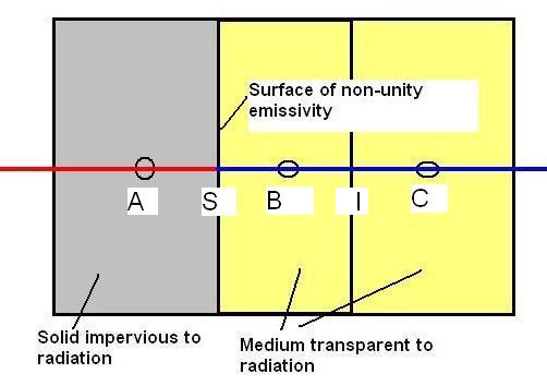
However, the calculation of the radiant flux at the S interface requires more careful study because the surface emissivity can cause a discontinuity of T3 gradient there, as is illustrated in the following figure, which shows the postulated profiles of both T3 and T1 because of their inescapable interaction.
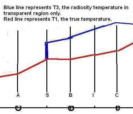
Here it is postulated that T3 and T1 are equal to each other within the solid but, whereas the latter has a finite gradient everywhere, the latter may have an infinite one at the interface between the phases.
The fluxes of energy in question are as follows:
qA-S = (T1,A-T1,S)/RA-S Eqn 15(b)
RA-S = (xS-xA)/λ1,A Eqn 15(c)
qc,S-B = (T1,S-T1,B)/Rc,S-B Eqn 15(d)
Rc,S-B = (xB-xS)/λ1,B Eqn 15(e)
qr,S-B = (T3,S-T3,B)/Rr,S-B Eqn 15(f)
Rr,S-B = (xB-xS)/λ3,B+(1-εS)/[εS4σT33] Eqn 15(g)
wherein the term involving εS is inserted so as to conform with equation (10) above.
qA-S = qc,S-B + qr,S-B Eqn 15(h)
and with T1S=T3S, the necessary formula can be deduced from eqn 15(h) as follows:
T1,S = T3,S = (T1,A/RA-S + T1,B/Rc,S-B + T3,B/Rr,S-B)/(1/RA-S+1/Rc,S-B+1/Rr,S-B) Eqn(16)
where the resistances RA-S, Rc,S-B and Rr,S-B were defined by equations 15(c), 15(e) and 15(g) earlier. Inspection of the Rr,S-B term in equation 15(g) shows that (xB-xS)/λ3,B is the conventional resistance and that (1-εS)/(εS4σT33) is the extra resistance caused by the non-unity emissivity.
From equations 15, 15(f) and 15(g) above, the radiative heat flux at the wall can now be written as:
qr,S-B = ΓS-B(T3,S-T3,B) Eqn (17)
where
ΓS-B = 4σT3,m3/[(xB-xS)(0.75(ε'+s')+1/Wgap) + (1-εw)/εw] Eqn (18)
and T3,m is a mean temperature between S and B, which is evaluated from:
T3,m3=(TS2+TB2)(TS+TB)/4 Eqn (19)
This expression follows from linearising the wall heat flux, as follows:
qr,S-B = σβ(TS4-TB4) = σβ(TS2+TB2)(TS2-TB2) qr,S-B = 4σβT3,m3(TS-TB) Eqn (20)
where by comparison with equation (18) above it is clear β is defined by:
β = [(xB-xS)(0.75(ε'+s')+1/Wgap) + (1-εw)/εw]-1 Eqn (21)
Few actions are needed in order to activate IMMERSOL. They comprise:
SOLVE(T3) to ensure that T3 is solved
DISWAL to activate the WDIS and WGAP calculation
STORE(WGAP) to enable this quantity to be accessed
together with such information as provides material properties and initial and boundary conditions.
Examples may be found in the IMMERSOL-related cases, in the advanced-radiation-option library.
From PHOENICS-3.4 onwards, however, the setting of radiation-related properties has been made more similar to the setting of other properties, such as density and specific heat.
Thus:
Moreover different values can then be placed in different parts of
the domain by the conventional use of:
FIINIT( ),
PATCH(name,INIVAL, ),
INIT(name, EMIS, ) and
INIT(name, SCAT, )
The differences from the treatment of other properties are:
Examples will be found in the input-library cases:
r201.htm,
r202.htm,
r203.htm and
r204.htm.
However, it should be noted that, when EMIS is set for a cell containing a
non-transparent solid, it becomes dimensionless; and it then represents the
emissivity/absorptivity of the surface of the solid.
(c) Domain-boundary conditions
Although the settings of EMIS within the transparent and non-transparent
media suffice to enable internal-to-the-domain boundaries to be
correctly represented, there is also sometimes a need to ascribe
radiation-influencing conditions at the boundaries of the domain.
For example, it may be desired to represent an aperture in the bounding surface, though which radiation can enter and leave; or a domain boundary may be required to simulate a solid wall of prescribed temperature, for which the emissivity must also be defined.
To meet this requirement, PHOENICS has been caused to react appropriately to PATCH and COVAL statements, for which the patch-name begins with the characters 'IM' and the dependent variable in question is T3.
How such patches are used is explained in the section of the lecture on IMMERSOL which may be viewed by clicking here,
(d) Wall-boundary conditions
At a wall boundary of known temperature and emissivity the following
boundary conditions are applied:
(a) PLATE
For a specified wall temperature and emissivity, the radiative heat flux at the wall is computed from:
qw = σβ(Tw4-T3,p4) = 4σβT3,m3(Tw-T3,p) Eqn (22)
where the wall resistance term β is given by:
β = [δ(0.75(ε'+s')+1/Wgap) + (1-εw)/εw]-1 Eqn (23)
and T3,m is a mean temperature between wall w and the near-wall node p, which is evaluated from:
T3,m3=(Tw2+T3,p2)(Tw+T3,p)/4 Eqn (24)
(b) Participating BLOCKAGE
Likewise, at the solid-fluid interface of a participating BLOCKAGE, the radiative heat flux at the wall for a specified emissivity is computed from:
qw = σβ(Ts4-T3,g4) = 4σβT3,m3(Ts-T3,g) Eqn (25)
where the wall resistance term β is given by:
β = [δ(0.75(ε'+s')+1/Wgap) + (1-εw)/εw]-1 Eqn (26)
and T3,m is a mean temperature between solid node and the fluid node g, which is evaluated from:
T3,m3=(Ts2+T3,g2)(Ts+T3,g)/4 Eqn (27)
(c) Non-participating BLOCKAGE
In PHOENICS 2018 and earlier, no action is taken at the adiabatic surface so that both the convective and radiative heat flux are zero.
In PHOENICS 2019 and onwards, both the radiative and convective heat flux are evaluated at the surface, and surface temperature is computed from the requirement that the total heat transfer rate is zero.
(d) THIN PLATE
The boundary conditions applied on either side of a thin plate are explained in detail here
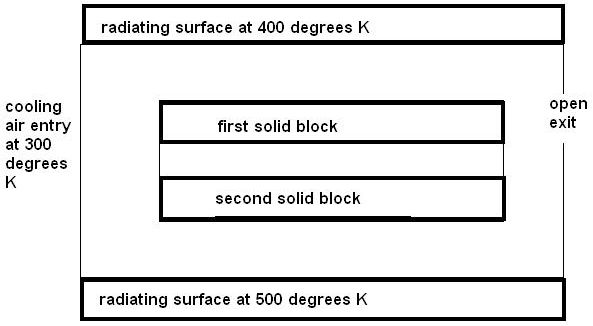
The practically interesting question is: What temperatures will be attained in the solid?
First some images showing the geometry and some results:

The grid and velocity vectors
The distributions of WGAP and of PRPS
The true (TEM1) and radiation (T3) temperatures
Since it is not easily seen from the above contour plot that TEM1 and T3 are very close within the solid, the following plot is provided of the difference between them. This is easily calculated by placing the following In-Form line in the Q1 file.
(stored tdif is tem1-t3)
The upward (y) and rightward (x) radiative heat fluxes
IMMERSOL has allowed this problem to be set up and solved with great ease, the advantage of which can be best appreciated by those who have attempted to solve such problems by the methods advocated in many text-books, involving use of 'view-factor' calculations.