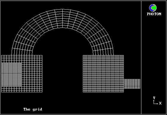
- a computational grid in a curved duct joining two box-shaped spaces;
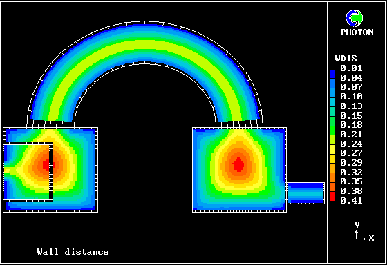
- the distance from the wall computed by the procedure to be described;
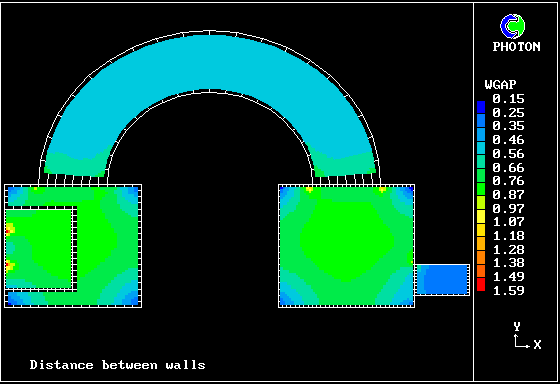
- the distance between the walls computed by the same procedure.
It must be understood that WDIS and WGAP have precise meanings only for especially simple circumstances, such as when the space between two wide parallel surfaces is considered. How they should be defined for points within a room cluttered with furniture is far from being obvious.
All that is claimed for the LTLS method is that it produces precisely correct values in the wide-parallel-plate circumstances; and results which are plausible in all others
Many turbulence models require the calculation, for every cell in the domain, of the distance from the nearest wall. They may also require the distance between the two nearest walls.
The Nikuradze mixing-length formula is an example.
Two-equation turbulence models such as k-epsilon have been invented for the purpose of making prescription of length scales unnecessary; but even they, in their low-Reynolds-Number forms, may require independent knowledge of distance from the wall for the evaluation of some terms.
One of the most convenient and (in PHOENICS) widely used if the IMMERSOL model. This also requires knowledge of the distribution in space of the distance between walls.
IMMERSOL therefore involves the solution of the feature.
The next three pictures represent:
Their inspection may lend credibility to the claims of plausibility which have just been made.
It is a convenient starting point for newcomers to the subject.
The LTLS feature involves the solution for a scalar variable, L, which:
within the fluid; and
This equation is similar to that for temperature within a uniformly-conducting medium, having a uniform heat source, and in contact with solids and other surfaces at which the temperature is held at zero.
It is of course easily solved by the linear-equation solver of PHOENICS, whether the geometry is one-, two- or three-dimensional. This solution needs to be determined once only, if the solids do not change position.
The variable L is not itself the distance from the wall, even though it is proportional to that distance at locations which are near a wall. Its dimensions are indeed those of length squared.
However, that distance can be deduced from the solution for L, as can also a plausible estimate of the effective distance between walls. The method is to derive a relationship between:
from consideration of a simple geometry, namely that between two parallel walls, and then to presumethat it has general validity.
Let the distance measured from one wall be y, and the distance to the opposite wall y1.
The differential equation takes the one-dimensional form:
d2L/dy2 = -1 , which can be integrated to give:
dL/dy = - y + A, where A is a constant, and then further to:
L = - y2/2 + Ay + B , where B is another constant.
Insertion of the boundary condition L=0 at y=0 and y=y1 yields:
B = 0 , and A = y1/2
with the result:
Elimination of y1 from the first equation by use of the second yields:
It is these equations which are employed generally.
They have been found to give plausible results in all situations; but of course, although Wdis has the unequivocal meaning of the distance to the nearest wall, the significance of Wgap has no clear meaning, in a corner for example.
It is interesting in this connection to consider a duct of circular cross-section; for it is again easy to obtain an analytical solution for L. The above equations then show that the above expression for Wdis is exactly correct in the immediate vicinity of the wall; and it rises to a maximum equal to radius divided by the square root of 2 at the centre of the duct.
Wgap, correspondingly, has the same value as the radius near the wall; and it rises at the centre of the duct to the radius times the square root of 2, i.e. exactly twice the reported distance from the wall.
How (and whether) the length scale of turbulence, LTURB, is to be deduced from WDIS and/or WGAP is of course a quite separate matter.
The model of Nikuradze, in which LTURB/WDIS is expressed as a poly-nomial in (WDIS/Wgap), is only one of many possibilities, of which another is to use the smaller of the Nikuradze formula and a length proportional to:
(maximum velocity - minimum velocity) / velocity gradient.
The following pictures illustrate the use of the model for the flow in a small element of a "labyrinth", i.e. a space in which fluid is forced to follow a winding path by the presence of solid obstacles.
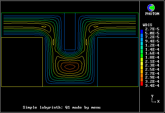
The wall distance
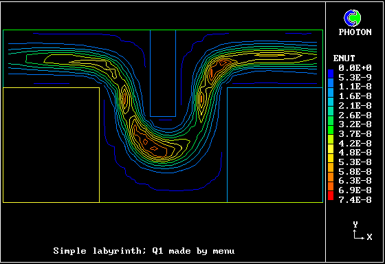
The effective viscosity
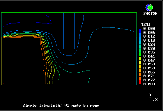
The temperature
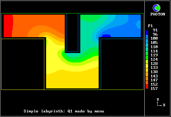
The pressure
See PHENC entries: DISWAL, LVEL, LAM-Bremhorst, and LOW-REYNOLDS NO.