At present, PLANT is capable of creating GROUND coding for:
Usually it will be non-linear relationships which will be provided by way of PLANT, because linear relationships can be introduced using PIL.
The coded relationships are normally used over the whole computational domain.
They can however be restricted to specific sub-domains and/or controlled by logical and relational conditions, by either REGION or PLACE and IF commands, where the latters are the special PLANT commands.
"labs"> PLANT reads statement lines in the Q1 file which begin with the tags:
Click here to return to "Contents"
The ?? wildcards represent a (section-consecutive) sequence number. This is one of the numbers up to 99 .
The lines must start in column 3 or more so that Satellite treats them as comments.
The remainder of the lines contain the formulae, or rather the relationships, provided by the user.
Dollar sign ($) as the last character on a line is treated as a continuation symbol.
PLANT also reads the next lines which contain COVAL, REGION or PLACE and IF commands.
These indicate how the formulae should be applied and together with statement lines form the PLANT instruction block.
REGION (IXF,IXL,IYF,IYL,IZF,IZL,ITF,ITL) { mark } / switch
It has 8 arguments, one parameter and one switch, namely (in order):
| IXF | index number of first cell in X-direction |
| IXL | index number of last cell in X-direction |
| IYF | index number of first cell in Y-direction |
| IYL | index number of last cell in Y-direction |
| IZF | index number of first cell in Z-direction |
| IZL | index number of last cell in Z-direction |
| ITF | index number of first time step |
| ITL | index number of last time step |
| mark | value of marker variable, MARK, of real type (optional) |
| switch | FORTRAN logical or relational expression (optional) |
PLACE (CXF,CXL,CYF,CYL,CZF,CZL,FT,LT) { mark } / switch
It has 8 arguments, one parameter and one switch, namely (in order):
CXF - coordinate of the west region boundary; CXL - coordinate of the east region boundary; CYF - coordinate of the south region boundary; CYL - coordinate of the north region boundary; CZF - coordinate of the low region boundary; CZL - coordinate of the high region boundary; FT - start time; LT - end time; mark - value of marker variable, MARK, of real type (optional); switch - FORTRAN logical or relational expression (optional).
Switch logical expression must have a syntax of FORTRAN construct and must be fully recognised by EARTH.
The permissible size of switch expression is confined by the length of the current REGION or PLACE command lines available, no continuation is allowed, so far.
The REGION or PLACE commands, if present, must immediately follow the {SC????} statements and COVAL command and start in column 3 or greater.
IF (logical expression).
The logical expression must have a syntax of FORTRAN construct and must be fully recognised by EARTH.
Its size is limited by the length of the current line available, no continuation is allowed, so far.
The IF command, if used, must follow immediately the COVAL, REGION or PLACE commands and start in column 3 or greater.
Then PLANT continues to read all strings as above until the end of Q1.
Afterwards PLANT edits the file GROUND.FOR to include the automatically generated FORTRAN coding, required for whatever expressions and conditions have been specified.
The FORTRAN which is coded accords with the rules of GROUND- Earth interactions.
1) the new GROUND must be compiled
2) a new Earth executable must be created
3) the new Earth must be run so as to perform the flow-simulation calculation.
These three operations are made automatically.
Any existing GROUND.FOR is copied to GROUND.SAV and a blank model GROUND.FOR is used as the starting-point for editing.
A copy of the code inserted is available for inspection in a file called PLTEMP.
Click here to return to "Contents"
PLANT permits specification of expressions in the Q1 file for DT, which is the name used to denote the values for the current time-step size in response of the pointer, TLAST=GRND
{SCTS??} DT={expression}
The PLANT block:
        {;SCTS01> DT=XG2D/U1
        REGION(NX/2,NX/2,NY/2,NY/2,NZ/2,NZ/2,2,2)
instruct EARTH to visit Group 2 of GROUND for a value of DT calculated within the sub-domain, in space and in time, indicated by arguments of REGION.
Further example.
Click here to return to "Contents"
PLANT permits specification of algebraic expressions in the Q1 file
for XRAT, YRAT and DZ which are the names used to denote the values
for:-
2.2 X-, Y-, and Z-direction grid specifications
Introduction of special grid specifications
To introduce special formulae for the grid steps, the user should
provide, in Group 3, and/or 4 and/or 5 of the Q1 file, lines
beginning with the tags:
{SCXS??} XRAT={expression}
{SCYS??} YRAT={expression}
{SCZS??} DZ={expression}
Some examples to be found in the PLANT Input File Library are as follows:
* for the current width of the domain:
      {SCYS01> YRAT=1.+:POWER:*DZ/(ZWADD+ZW)
      REGION(1,1,1,1)
      IF(IZ.LE.20)
* for forward step size:
     {SCZS02> DZ=DZL*(1.-0.02*TEMP[,1,-1]/:TJET:)
     IF(IZ.GT.2)
The statement
{SCYS01> YRAT=1.+0.5*DZ/(RG(1)+ZW)
gives the dependence similar to laminar boundary layer near the flat plate, where The RG is PIL-set parameter.
If the problem is stated in the X-Y plane, user should perform an exactly corresponding actions for the X-direction domain width, XULAST, so that performed above for XULAST using AZYV=GRND as a pointer, {SCXS??} as a tag and XRAT as variable name of the statement.
The following block may be used to make the step size DZ a fixed fraction, RG(1), of the calculation domain width XULAST in parabolic calculations for all IZ-slabs greater or equal to 5 when the number of cells in X-direction is greater than unity.
      {SCZS01> DZ=RG(1)*XULAST
      REGION(1,NX,1,NY,5,NZ,1,1)
      IF(PARAB.AND.NX.GT.1)
Further examples of expanding/contracting and adaptive grids .
Click here to return to "Contents"
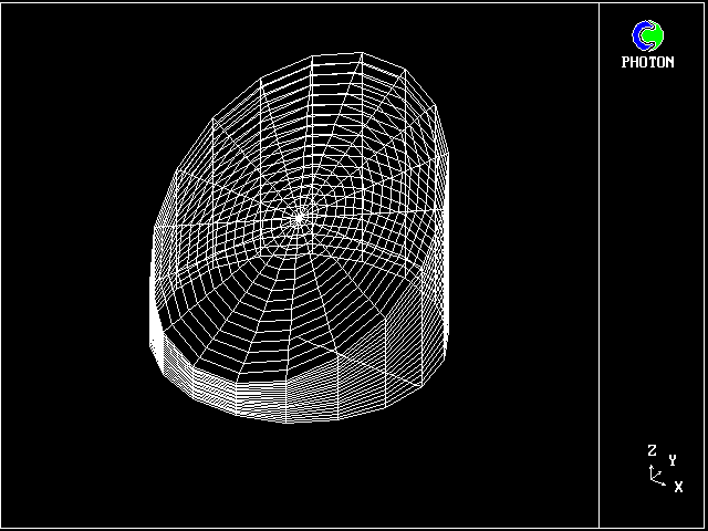
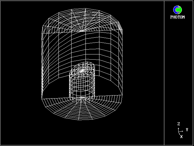
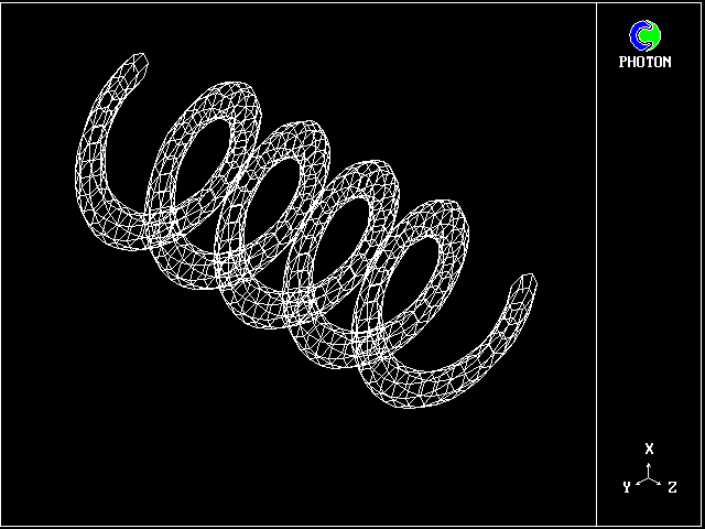
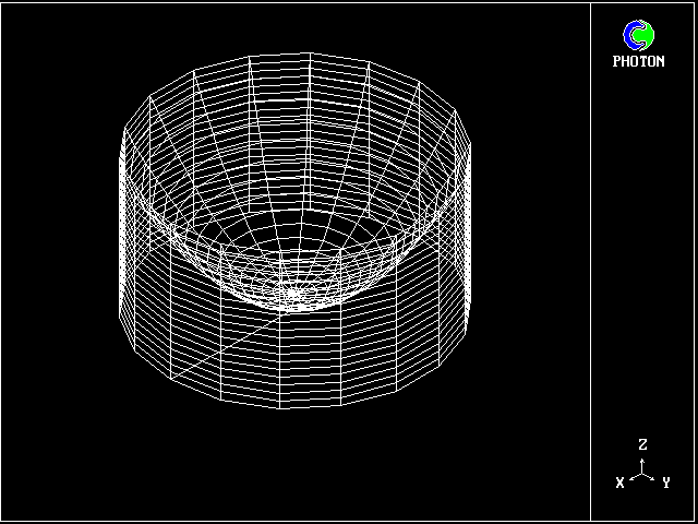
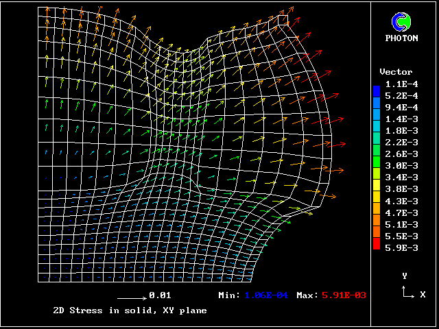
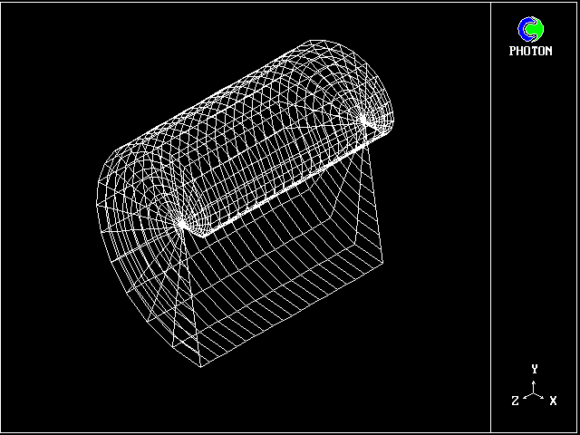
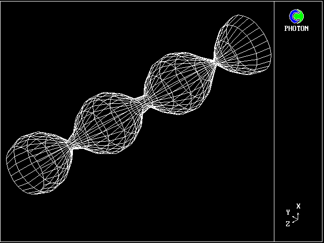
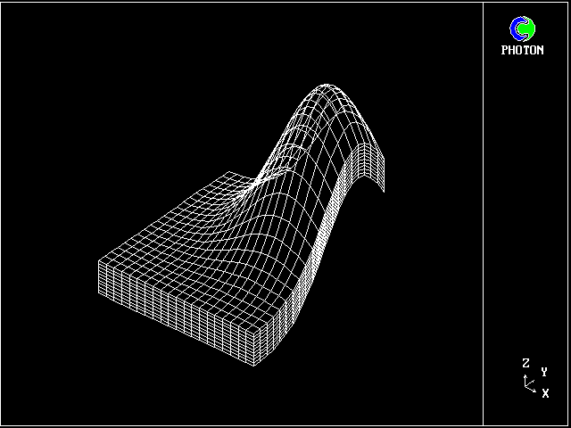
When BFC equals T in Q1 file, user can introduce the formulae to calculate the corner coordinates of a body-fitted grid to create the geometry and corresponding grids by way of parametric analitics. PLANT therefore provides the possibility of amending these geometrical entities, say with time.
PLANT will place the corresponding codings in Section 2 of Group 19 of GROUND.FOR so that the geometry can be changed in accordance with time at first sweep for all time steps.
The format of PLANT statements in Q1 Group 6 is as follows
{MXYZ01> XC= { expression }
{MXYZ01> YC= { expression }
{MXYZ01> ZC= { expression }
where the tags {MXYZ??} tell PLANT that the corresponding expressions should be coded to calculate the cartesian coordinates, XC, YC and ZC, of the corners of continuity cells.
BFC=T
REAL(LITTLER,TWOPI)
LITTLER=1.0;TWOPI=2.0*3.14157
NX=8;NY=6;NZ=1
{MXYZ01> XC=:LITTLER:*FLOAT(J-1)/FLOAT(NY)*$
COS(:TWOPI:*FLOAT(I-1)/FLOAT(NX))
{MXYZ01> YC=:LITTLER:*FLOAT(J-1)/FLOAT(NY)*$
SIN(:TWOPI:*FLOAT(I-1)/FLOAT(NX))
{MXYZ01> ZC=FLOAT(K-1)/FLOAT(NZ)
CSG1=PHI;CSG2=XYZ
set the BFC grid for a circle of unity radius in XY plane. The corner coordinates will dumped to X1 file and calculation results to P1 file for examination via PHOTON.
Further examples of analytical grid generation including moving BFC option are illustrated below.
Example 1, 2, 3, 4, 5, 6, 7, 8, 9, 10.
Click here to return to "Contents"
PLANT permits specification of algebraic expressions in the Q1 file for extra velocities to be added to their current slab store at the point in the computation at which the convection fluxes are assembled. The pointers U1AD, U2AD, V1AD, V2AD, W1AD and W2AD must be set to GRND, as appropriate.
{SCUF??} VELAD = { expression
for 1st phase U1 extra velocity}
{SCUS??} VELAD = { expression
for 2nd phase U2 extra velocity}
{SCVF??} VELAD = { expression
for 1st phase V1 extra velocity}
{SCVS??} VELAD = { expression
for 2nd phase V2 extra velocity}
{SCWF??} VELAD = { expression
for 1st phase W1 extra velocity}
{SCWS??} VELAD = { expression
for 2nd phase W2 extra velocity}
        {SCUF01>  VELAD = U2
        {SCVF01>  VELAD = V2
        {SCWF01>  VELAD = W2
Further example of convection fluxes alteration.
Click here to return to "Contents"
PLANT permits specification of expressions in the Q1 file for:
In addition, the pointers TMP1, TMP2, EL1, EL2, RHO1, RHO2, DRH1DP, DRH2DP, ENUL, ENUT, PRNDTL(PHI) and PHINT(PHI) must be set to GRND, as appropriate.
{PRPT??}
* for laminar viscosity:
     {PRPT01>   VISL=0.001*EXP(-1.6*(TEMP-0.0))
     {PRPT02>   VISL=EMU/DEN1
* for laminar Prandtl Number:
{PRPT03> LAMPR(H1)=EMU*CP/COND
* for turbulent viscosity:
{PRPT01> VIST=1.6/7.*YG2D**1.142/100.**0.142
* for length-scale of turbulence:
{PRPT01> LEN1=DIST
* for phase interface values
{PRPT01> FII1(H1)=H2
   RHO1 = GRND
      {PRPT1>  DEN1 = 1./H1
   ENUL = GRND

      {PRPT2>  VISL = RG(1)*SQRT(TEM)
   PRNDTL(H1) = GRND
      {PRPT3>  LAMPR(H1) = VISL*DEN1*RG(2)*RG(3)
Here RG(1), RG(2) and RG(3) are used to transfer to GROUND the values of constants used in the property expressions.
Further examples of a non-linear property correlations.
Click here to return to "Contents"
PLANT permits specification of linear or non-linear inter-phase data including:
The pointers CFIPS, CMDOT, and CINT(PHI) must be set to GRND, as appropriate.
{PRPT??}
     {PRPT1>   COI1 (H1) =10. *MASS2
     {PRPT2>   FII1  (H1) = H2
     {PRPT3>   FII2 (H2)  = H1
     {PRPT1>   INTFRC=500.*R2*MASS1
The following block inserted in Group 10 of Q1 effects this dependence:
   CF1PS = GRND
       {PRPT1>  INTFRC = CFIPA*MASS1*R2
PLANT supplies similar options for CMDOT and CINT(PHI) as further examples show.
Click here to return to "Contents"
Some examples to be found in the input-file library now follow.
From library case 19:
   PATCH(INIT,INIVAL,1,NX,1,NY,1,NZ,1,1)
        {INIT01>  VAL=XG2D+YG2D
   INIT (INIT,C1,0.0,GRND)

         {INIT02>  VAL=XG2D*YG2D
   INIT (INIT,C2,0.0,GRND)
   PATCH(LASTHALF,INIVAL,1,NX,1,NY,NZ/2,NZ,1,1)
     {INIT1>  VAL = RG(1)+RG(2)*YG2D+RG(3)*YG2D**2
   INIT(LASTHALF,W1,0.0,GRND)
instructs EARTH to visit Group 11 of GROUND for an array of values for the field of W1 at each slab within the sub-domain indicated by arguments 3 to 8 of PATCH.
The line headed by {INIT??} and corresponding INIT commands must not be separated by blank or comment lines.
The number of devices for initialisation of variables and porosity fields can be implemented by this way.
Click here to return to "Contents"
PLANT facilitates the building up of sophisticated non-linear sources and boundary conditions. This is done by way of formulae from which the CO and VAL of COVAL commands are computed cell-by-cell and sweep-by-sweep, as the flow-simulation proceeds.
     {SORC01>   VAL=TIM+YG2D
     {SORC02>   VAL=TIM+1.0+YG2D
     {SORC03>   VAL=TIM+XG2D
     {SORC04>   VAL=TIM+1.0+XG2D
     {SORC05>   VAL=TIM+XG2D+YG2D
     {SORC01>   CO=C1**3*TIM**3
     {SORC01>   CO=RG(1)
The following blocks instruct PLANT to create the necessary coding, and EARTH to look for an array of VALues and/or COefficients for the PATCH:
   PATCH(HEAT,VOLUME,3,7,2,20,3,6,1,1)
     {SORC01>  VAL = RG(1)*XG2D+RG(2)*YG2D+RG(3)*ZGNZ
   COVAL(HEAT,H1,FIXFLU,GRND)

   PATCH(INLET,LOW,1,NX,1,NY,1,1,1,1)
     {SORC02>  VAL = RG(1)*(RG(2)+RG(3)*YG2D+RG(4)*YG2D**2)
   COVAL(INLET,P1,FIXFLU,GRND)
     {SORC03>  VAL = RG(2)+RG(3)*YG2D+RG(4)*YG2D**2
   COVAL(INLET,W1,ONLYMS,GRND)

   PATCH(BAFFLE,PHASEM,1,NX,1,NY,1,NZ,1,1)
     {SORC04>  CO = RG(1)*U1**(RG(2)-1.)
   COVAL(BAFFLE,U1,GRND,0.0)

     **  Heat exchange between lower  and upper sub-domains
   PATCH(HEATEXT1,VOLUME,1,NX,1,NY,1,NZ,1,1)
     {SORC10> CO =RG(1)*(U1**2+V1**2+W1**2)**0.4
     {SORC10> VAL=TEM2
   COVAL(HEATEXCH,TEM1,GRND,GRND)
       **  Heat exchange between upper and lower sub-domains
   PATCH(HEATEXT1,VOLUME,1,NX,1,NY,1,NZ,1,1)
     {SORC11> CO =RG(2)*(U2**2+V2**2+W2**2)**0.4
     {SORC11> VAL=TEM1
   COVAL(HEATEXT1,TEM2,GRND,GRND)
There must be neither comments no blank lines both between headed lines
and between them and COVAL command. The following PLANT block is
therefore invalid:
Click here to return to "Contents"
PLANT also permits the introduction of coding into the various
sections of Group 19 of GROUND allowing re-calculation of selected
variables, intervention in calculations and special output
preparations.
These may prevail for the whole or part of the domain in space and in
time ( by use of REGION or PLACE commands) and can be conditionally
controlled (by IF command).
Example 1: which computes the distance from the wall.
Example 2: User-specified output
The next example concerns the following
statements of PLANT block which are
needed to calculate the Nusselt number, Nu, over part of the south
wall for a uniform grid, in Group 19, Section 6, at the finish of the
IZ-slab:
It should be noted that NORTH(TEM1) denotes the north value of
TEMperature and instructs PLANT to make the coding access the
north neighbours of the specified REGION.
The SOUTH(PHI), EAST(PHI), WEST(PHI), HIGH(PHI), LOW(PHI) and
OLD(PHI) perform the corresponding functions in the other co-ordinate
directions.
Further examples of output control
settings and special calculations.
Click here to return to "Contents"
PLANT permits specification of algebraic expressions in the Q1
file for RESREF(PHI) which is the reference value of residual for
the variable indicated.
{SCnn??} RESREF(PHI) ={ expression }
where nn is user specified Section number of Group 19.
The block:
instructs EARTH to visit Section 3 of Group 19 of GROUND for a value
of RESREF(W1) calculated within the sub-domain, in space and in time,
indicated by arguments of
REGION.
Click here to return to "Contents"
PLANT permits specification of expressions
in the Q1 file for DTFALS(PHI) which is the value of false-time-step of
under-relaxation for the variable indicated.
{SCnn??} DTFALS(PHI) ={ expression }
where nn is user specified Section number of Group 19.
The block:
instructs EARTH to visit Section 6 of Group 19 of GROUND for a value
of DTFALS(H1) calculated within the sub-domain, in space and in time,
indicated by arguments
of REGION.
Further examples of setting under-relaxation
devices.
Click here to return to "Contents"
PLANT permits specification of expressions
in the Q1 file for VARMAX(PHI) and VARMIN(PHI) which are the maximum
and minimum values allowed to variable indicated.
If VARMAX(PHI) is less than -1.e-10, it will be treated as the
maximum absolute value of the increment of the value at any updating
stage.
If VARMIN(PHI) is less than -1.e-10, it will be assumed that the
absolute change made to the variable at all updating stages is
limited to VARMAX.
{SCnn??} VARMAX(PHI) ={ expression }
and/or
where nn is user specified Section number of Group 19.
The block:
instructs EARTH to visit Section 6 of Group 19 of GROUND for a value
of DTFALS(H1) calculated within the sub-domain, in space and in time,
indicated by arguments of REGION.
Further example of setting limits and
increments.
Click here to return to "Contents"
For global summation PLANT inserts Ground coding in Groups 2-5, 8 and
19 which will calculate a single value or a number of values as a
result of summating over the whole domain (or over a specified part
of the domain) for the expression
specified as the argument.
The calculated value(s) are put into a file called globcalc and labelled.
VAR = SUM (
expression),
where VAR stands for automatically declared user real variable name.
In the above, the line headed {SC0601> contains the variable R, to be
computed and the algebraic expression which is summed over the extent
of the domain as specified by the REGION
command. For the case shown, R will be the sum of the magnitude of
the velocities in the XY plane.
The command {TEXT> transmits up to 30 characters of text which will be
printed in the globcalc file as,
Global summation feature has proved to be useful in many actions
beyond its primarily function, as exemplified for
time specification case.
Click here to return to "Contents"
Using the above procedure, PLANT permits properties, sources and
solid objects to be placed within pre-defined grids, their presence
being signalled by the attachment of the corresponding fluxes and
material-property values to the appropriate cells.
The grid can be cartesian, polar or BFC one, the fineness of which
the user can control; but he concerns himself only with the
construction of the cell-wise distributions of variable, MARK, which
constitute the shapes of the MARKed regions.
A library of utility functions is
available for calculation of marker distributions in the flow
domain. The latters are used to represent the inserts of complex
shapes, moving objects, solid shape distortions, region
identifications etc.
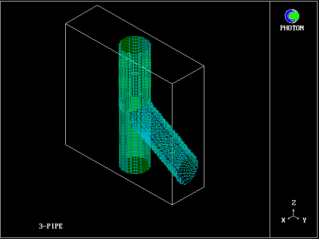
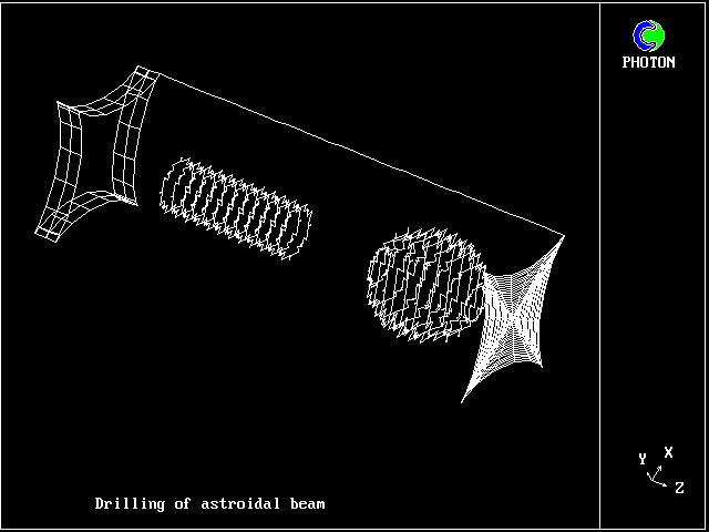
will "drill" the circular tube from one corner of the cube to the
opposite one. Other operations, which make cavities having plane
surfaces, have an effect similar to the operation of a milling machine.
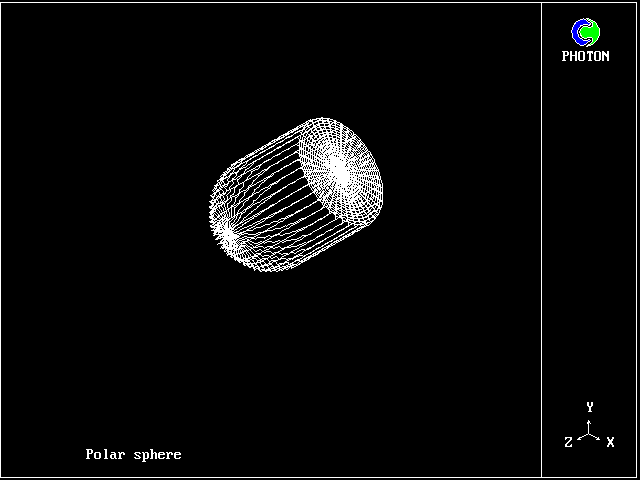
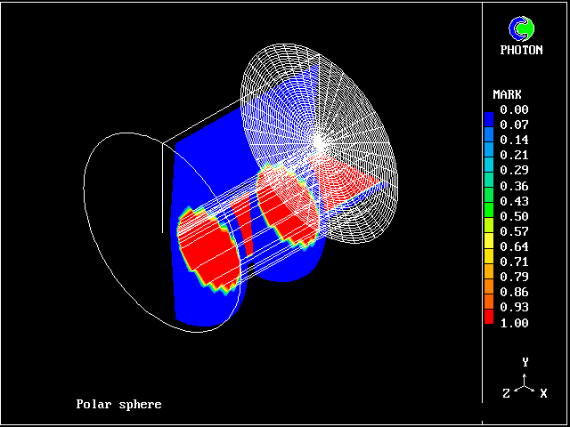
In above settings the coordinate arguments of SPHERE function vary
with X direction coordinate. For uniform grid it makes the SPHERE
function to "drill" the circular diagonal pipe of 2.5 diameter in a
cube the cells of which are marked by MARK=1. Each cell of the pipe
has the marker MARK=0.0.
Here, the function XYBOX is used to calculate time varying
re-location of unity object MARKer ( 1st argument) as a linear
function of current time and object velocity, RG(1), ( 2nd argument
expression). The next three arguments set the cartesian coordinate
of south-west box corner and the sizes of its sides. The sixth and
seventh arguments, representing rotation angles, are zeros here.
By this technique, the regions of various shapes can be marked and
use for introduction of material properties, sources, intervention
in the calculations and processing the results.
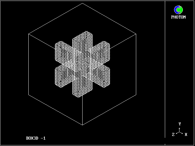
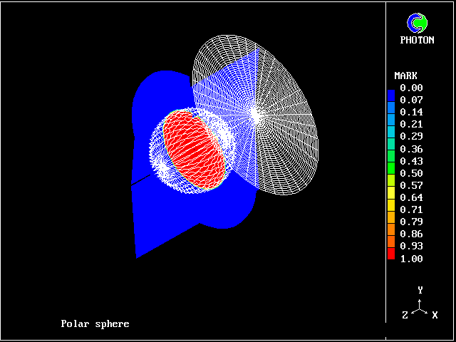
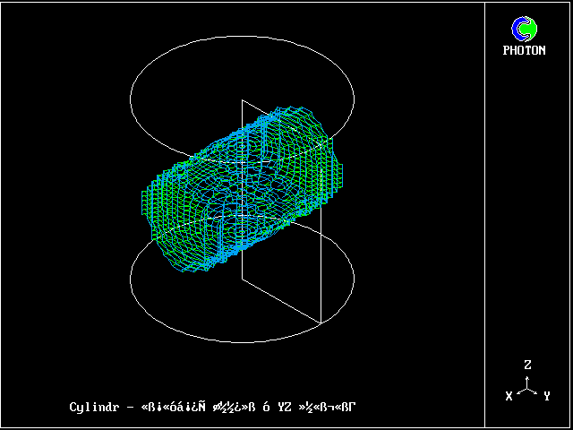
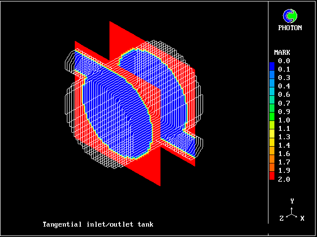
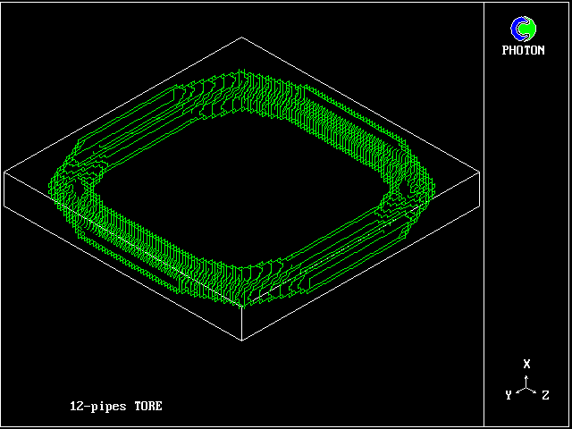
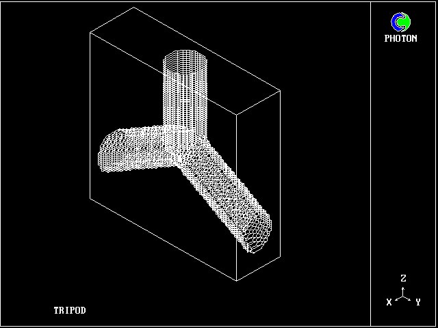
At present, eight classes of functions are available. They are:
Many shapes of arbitrary complexity can be generated by combinations
of above functions in planted expressions as exemplified for field
initialisations. The number of further
examples are shown below.
Click here to return to "Contents"
There are PLANT options which are aimed to provide the users with the
means to plant the specific codings in a flow domain regions defined
in terms of physical space coordinates rather than grid ones.
The following four ways to make grid-free planting are permitted:
(1) Using PLACE command
It is the most straightforward way because command
PLACE is
nothing more than conditional grid-free variant of PATCH.
(2) Using marker distribution
PLANT can use the grid free distribution of the marker, MARK,
over the flow domain as a series of objects fitted in the
arbitrarily specified cartesian grid.
The coding which is then PLANTed in GROUND contains logic for
the mathematical expression to be tied up with the regions
filled by the specific marker property.
The syntax of PLANT instructions for PATCH, COVAL and
REGION commands is as follows
(i) For PATCH/COVAL combinations
Here SS ( Space Source ) stands for special PATCH name
characters, mrk stands for the value of MARK variable used to
define the region over which
expressions should be applied and
the last three characters, NAM, can be used arbitrarily.
Note that PATCH arguments are applied for the whole domain, not
for a part of it.
(ii) To cause PLANT to perform grid free codings in Group 19
the REGION command should
be with parameter
where mrk stands for marker, MARK, value.
The following block
provide the application of expression for variable HEAT at the
end of the iz-slab for the part of the flow domain marked by
MARK=100.
(3) Over-writing PATCH arguments by parameterized
REGION command
The following block initialises
PRPS field to 100 over the extent of the PATCH where MARK
is equal to unity
is equivalent to
where whole field extent of the PATCH named IN is brought in
conformity with SS001IN PATCH extents by way of
REGION command with unity parameter.
(4) How to make the extents of the PATCHes grid-free
The foregoing example shows that the combination of PIL and PLANT
commands can be used to change the extents of the PATCH. The example
below shows how to replace the PATCH limits by extents in physical
space.
If it is desired to replace the grid arguments of PATCHed source by
grid-free limits, one can use the combination of PATCH, COVAL and
PLACE commands as the following
block shows:
The result will be that source for U1 calculated as GRDm option of
COefficient and GRNDn option for VALue will be applied over the
extent of 0.0 to 1.0m in X-direction, 2.0 to 5.6m in Y-direction,
0.45 to 3.0m in Z-direction and 1.0 to 2.0s of time.
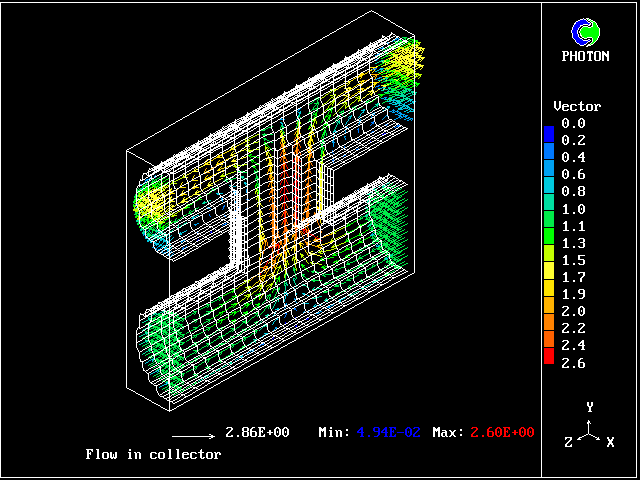
The multi-space, HEXAGON, model for
Solid-Fluid-Thermal analysis of heat exchanger performance provides
rather typical example of the grid-free operations.
Click here to return to "Contents"
PLANT allows for mathematical expressions
to be planted into the GROUND to operate straightforwardly with
either in-cell or its nearest neighbours, i.e. " old", "high", "north"
and "east" field variables referenced by their names, OLD(PHI),
HIGH(PHI) etc. as the example below shows.
PLANT is also taught to work not only with fixed elements of
PHOENICS global F-array. PLANT can manipulate whole segments of
array which contain variables of defined class. The latter feature
greatly facilitates the building up sophisticated indicial
expressions which otherwise would require in-depth knowledge of
GROUND-EARTH-SATELLITE interior connections and number of special
rules and techniques.
The built-in technique employs efficient procedural operators to
build indexed expressions right in Q1. This is done by way of
straightforward using of cell-location-coordinate indices in three
coordinate directions instead of their linear functions as for
conventional GROUND coding.
Some examples of how to handle indices now folllow.
Many developments may require above feature, as exemplified for
field initialisation.
Click here to return to "Contents"
PLANT commands can make use of additional
information about what the user wants to do. This information may be
included by typing-in the parameter after
typed command. Usually, the command will have a default - it will
automatically perform its function in certain way if there is not
typed-in parameter.
The LG(1) switch specifies that the
relationship, DEN1=1./H1, will be used if LG(1)=T appears
somewhere in Q1.
Simple logical expressions can be combined with the logical
operators .AND.,.OR. and .NOT. to create arbitrary complex logical
switches:
The switches allows the compact way to introduce short relational
and logical conditions in PLANTed coding.
However, it is, sometimes, more convenient to use special command
for introduction of IF ... THEN construct. The
IF command ensures that the longer valid
logical expression used as command argument conforms the correct
FORTRAN planted in the right place.
       PATCH(SS111B,TYPE,1,NX,1,NY,1,NZ,1,TLAST)
         {SORC77> CO  = { expression }
           Invalid comment: Above are the formula for COefficient
         {SORC77> VAL = { expression }
           Invalid comment: Above are the formula for VALue
       COVAL(SS111B,U1,GRND,GRND)
2.9 Special calculations and output control
Introduction of special calculations
To introduce special calculations, the user should provide, anywhere
of the Q1 file, statement lines beginning with the
tags:
When resulting coding is planted into Section 6, for example, which
corresponds to the finish of all operations on the current IZ-slab,
it allows the building of user own arrays of (say) Nusselt numbers
patch-wise, and then print them graphically, or inspect on the
screen.
Examples from the library
   ** The distance to the nearest wall
         DIST=sqrt((grad L)**2 + 2.*L) - grad L
   STORE(DLDZ,DLDY)
     {SC0601> DLDZ=(HIGH(LTSL) - LOW(LTSL))/(2.*DZGNZ)
        REGION(1,1,1,20,2,19)
     {SC0602>  DLDZ=(HIGH(LTSL) - LTSL)/DZGNZ
        REGION(1,1,1,20,1,1)
     {SC0603>  DLDZ= (LTSL - LOW(LTSL))/DZL
        REGION(1,1,1,20,20,20)
     {SC0604>  DLDY=(NORTH(LTSL) - SOUTH(LTSL))/(2.*DYG2D)
        REGION(1,1,1,1,1,20)
     {SC0605>  DLDY=(NORTH(LTSL) - LTSL)/DYG2D
       REGION(1,1,1,1,1,20)
     {SC0606>  DLDY=(LTSL - SOUTH(LTSL))/SOUTH(DYG2D)
       REGION(1,1,20,20,1,20)
     {SC0607>DIST=SQRT(DLDZ**2+DLDY**2+2.*LTSL)-SQRT(DLDZ**2+DLDY**2)
       REGION(1,1,1,20,1,20)
   STORE(NU)
   INTEGER(IX1,IX2)
   IX1 = 3; IX2 = 6
     {SC061> NU=RG(1)*ABS(TEM1-NORTH(TEM1))/YG2D
     REGION(:IX1:,:IX2:,1,NY/2,1,NZ,1,1)
2.10 Reference residuals
Introduction of reference residual
To introduce reference residual formulae, the user should provide, in
the Q1 file, lines beginning with the tag:
An example of reference residual specification
An example is the calculation of the reference residual for W1 at the
start of each Z-slab as momentum flux at the midlle-domain cell.
        {SC0301> RESREF(W1)=AHIGH*DEN1*W1**2
        REGION(NX/2,NX/2,NY/2,NY/2,NZ/2,NZ/2,1,1)
2.11 Under-relaxations
Introduction of under-relaxation
To introduce under-relaxation formula, the user should provide, in
the Q1 file, lines beginning with the
tag:
An example of under-relaxation
An example is the calculation of the under-relaxation for H1 at the
start of each Z-slab as residence time for the midlle-domain cell
velocity. It should be applied for the time moments greater than 2.
        {SC0601> DTFALS(H1)=ZWLAST/W1
        REGION(NX/2,NX/2,NY/2,NY/2,NZ/2,NZ/2,2,LSTEP)
2.12 Limits on variables and increments to them
Introduction of limits and increments
To introduce limits and increments formulae, the user should provide,
in the Q1 file, lines beginning with the
tag:
{SCnn??} VARMIN(PHI) ={ expression }
An example of limits and increments
An example is the calculation of the maximum value allowed to H1 at
the start of each Z-slab as its middle domain value. It should be
applied for the time moments greater than 2.
      {SC0601> VARMAX(H1)=H1
      REGION(NX/2,NX/2,NY/2,NY/2,NZ/2,NZ/2,2,LSTEP)
2.13 Global summation
Introduction of global summation
The function SUM has the syntax:
An example of global summation
   {SC0601>R=SUM(SQRT(U1**2+V1**2))
   {TEXT>Variable R
   REGION(1,NX-1,1,NY-1,1,1)
   Global Calculations:
   Variable R           = 4.70132
2.14 Marker Allocation Procedure
Introduction of marker allocations
User is helped in the performance of marker allocations by
sufficiently varied set of special functions, the selection, sizing and
location of which are the user's main tasks.
An example of marker allocation
The next settings
    FIINIT(MARK)=1.0
    PATCH(INI1,INIVAL,1,NX,1,NY,1,NZ,1,1)
      {INIT01> VAL=SPHERE(0.,XG2D,XG2D,XG2D,2.5)
    INIT (INI1,MARK,0.,GRND)
A further example of marker allocation
This is concerned with marker allocation for moving object:
    {SC0304> MARK =XYBOX(1.0,RG(1)*(TIM-1.),48.,30.,30.,0.0,0.0)
    IF(ISWEEP.EQ.1)
Further information
name shape orientation
BOX rectangular box any
ELLPSD ellipsoid any
SPHERE sphere any
XYBOX rectangular box XY plane
XYCIRC circle XY plane
XYELLP ellipsoid XY plane
XYWEDG triangular wedge XY plane
YZBOX rectangular box YZ plane
2.15 The grid-free operations
         PATCH(SSmrkNAM,TYPE,1,NX,1,NY,1,NZ,1,LSTEP)
           {SORC01> CO  = { expression }
           {SORC01> VAL = { expression }
         COVAL(SSmrkNAM,V1,GRND,GRND)
REGION(1,NX,1,NY,1,NZ,1,LSTEP ) {mrk}
         {SC0608> HEAT= { expression }
         REGION(1,NX,1,NY,1,NZ,1,LSTEP) 100
         PATCH(SS001IN,INIVAL,1,5,2,3,8,20,1,LSTEP)
           {INIT32> VAL=100
         INIT (SS001IN,PRPS,0.,GRND)
         PATCH(IN,INIVAL,1,NX,1,NY,1,NZ,1,LSTEP)
           {INIT32> VAL=100
         INIT (IN,PRPS,0.,GRND)
           REGION(1,5,2,3,8,20,1,LSTEP) 1
     SOLVE(P1,U1,V1)
     STORE(DUMMY)
     REAL(ANYVALUE);ANYVALUE=1234.
     PATCH(ZZZ,CELL,1,NX,1,NY,1,NZ,1,LSTEP)
     COVAL(ZZZ,U1,GRND3,GRND3)
       {SORC01> CO = ANYVALUE
     COVAL(ZZZ,DUMMY,GRND,ANYVALUE)
       PLACE(0.,1.,2.,5.6,0.45,3.0,1.,2.)
2.16 Indexed Variable Operations
          {SC0601> NU=RG(1)*ABS(TEM-NORTH(TEM))/YG2D
          REGION(1,1,1,NY,1,NZ,1,1)
An example of fixed indices
Examples of indices relative to the current cell location
   Index        PHOENICS          PLANT
  required  integer function     operand

     P          -               PHI or PHI[,,]
     E       EAST(PHI)          PHI[+1,,]
     N       NORTH(PHI)         PHI[,+1,]
     H       HIGH(PHI)          PHI[,,+1]            NN      HH
     W          -               PHI[-1,,]            |     /
     S          -               PHI[,-1,]       NW   N   H
     L          -               PHI[,,-1]          / | /
     EE         -               PHI[+2,,]     WW--W--P--E--EE
     NN         -               PHI[,+2,]          / | /
     HH         -               PHI[,,+2]        L   S   SE
     WW         -               PHI[-2,,]      /     |
     SS         -               PHI[,-2,]    LL      SS
     LL         -               PHI[,,-2]
     NW         -               PHI[-1,+1,]
     SE         -               PHI[+1,-1,]
     and so on...
A further example
The following PLANT block placed in Q1
file provides the calculations of pressure field at each IZ-slab
relative to the pressure at the cell of IX=1, IY=1 and IZ=1.
            STORE(PNEW)
              {SC0601> PNEW=P1-P1[1,1,1]
2.17 Logical and conditional operations
An example of command switch
If PLANT is used to make the first-phase density being reciprocal to
the first-phase enthalpy for the whole domain up to third time
moment inclusively, but only when LG(1)=T in Q1, the following
block of instructions should be typed-in:
       RHO1=GRND
         {PRPT01> DEN1=1./H1
         REGION(1,NX,1,NY,1,NZ,1,3) /LG(1)
     REGION(1,NX,1,NY,1,NZ,1,3) /LG(1).AND.ISWEEP.EQ.LSWEEP-10
     REGION(1,NX,1,NY,1,NZ,1,3) /IX.GT.NX-10.AND..NOT.BFC
An example of IF command
The command with switch
REGION(1,NX,1,NY,1,NZ,1,3) /IX.GT.NX-10.AND..NOT.BFC
is equivalent to:
       REGION(1,NX,1,NY,1,NZ,1,3)
       IF(IX.GT.NX-10.AND..NOT.BFC )
Further typical examples.