The domain-partitioning technique is useful for computer simulation of flow phenomena characterised by a predominant direction of flow, as for example when several chemical-plant vessels are connected in series, as sketched below, the flow being always from left to right.
It is of course possible, with sufficient computer memory, to simulate all three vessels, and the pipes and spaces between them, at the same time; but it is seldom either necessary or cost-effective to do so; for there is usually no significant influence of happenings in downstream vessels on those in upstream ones.--------------- --------------- ------------- | | | | | | | | | | | | - vessel 1 ---------- vessel 2 --------- vessel 3 --------- - ---------- --------- --------- | | | | | | | | | | | | --------------- --------------- ------------- upstream >>>>>>> direction of flow >>>>>>>> downstream
A similar situation arises when it is necessary to simulate the flow over an extensive tract of terrain, for example a complete city or a wide forest. Partitioning is then possible because usually the direction of wind varies little from place to place.
Thus, if the wind blows predominantly from the north west over the area of land indicated below, the sub-areas marked 1, 2, 3, etc. below can be simulated separately but in sequence, if the output from an earlier calculation is stored for use as input to a later one.
  \
   \
    \   wind from
     _| north-
         west               North
      |----------|---------|---------|---------|--------|--------|---
      |          |         |         |         |        |        |
      |    1     |   2     |   3     |    4    |   5    |   6    |
  West|          |         |         |         |        |        |
      |          |         |         |         |        |        |
      |----------|---------|---------|---------|--------|--------|---
      |          |         |         |         |        |        |
      |    7     |   8     |   9     |    10   |   11   |   12   |
      |          |         |         |         |        |        |
      |          |         |         |         |        |        |
      |----------|---------|---------|---------|--------|--------|---
      |          |         |         |         |        |        |
      |    13    |   14    |   15    |    16   |   17   |   18   |
      |          |         |         |         |        |        |
      |          |         |         |         |        |        |
      |----------|---------|---------|---------|--------|--------|---
When it is desired to take into account the shapes of individual buildings in the city, or of fire-breaks traversing the forest, the computer-memory requirements could not be met by commonly-available machines if the whole region were to be simulated at once.
The domain-partitioning technique however does permit the simulation to be performed by computers of modest size.
It does so by splitting the whole terrain into parts which are sufficiently small to be handled by the available computer; and it then causes the parts to be simulated one after the other, the upwind ones being considered first.
At the end of each calculation, data describing the flow conditions on the downstream boundaries are placed into files which serve as 'transfer objects'; for the data can then be transferred by export to, and import by, the later-to-be-simulated next-downstream part.
The first causes the PHOENICS solver module, EARTH, to write a transfer-object file at the end of its run; and the second causes EARTH to read such a file at the start of its run.
The advantage of using the 'object' concept for transmission of the data is that it is grid-independent. Thus there is no need for the grid employed for the exporting calculation to conform with that of the importing one.
(EXPORT to NAME_OF_TRANSFER_OBJECT at PATCH_NAME)
wherein
NAME_OF_TRANSFER_OBJECT
and
PATCH_NAME are
respectively:
Names of transfer objects should not exceed 14 characters.
The reading of the information from a transfer-object file is effected by placing in the Q1 file an In-Form (import statement such as:
(IMPORT from NAME_OF_TRANSFER_OBJECT at PATCH_NAME)
For this reason, the location of the transfer object is conveyed by associating it with a VR object of PLATE type, which is located by way of the usual POSITION and SIZE lines.
The (export and (import statements then take the form:
(EXPORT in NAME_OF_TRANSFER_OBJECT at OBJECT_NAME)and
(IMPORT in NAME_OF_TRANSFER_OBJECT at OBJECT_NAME)Input-library case 864 provides an example.
Note added in July, 2010
Subsequent to the first introduction of transfer objects, three
new PHOENICS capabilities have been introduced which may permit the
transfer-object feature to be further improved in the future. They are:
-
Had these been available when transfer objects were invented, it would
have been simpler to use then rather than the VR PLATE object.
Thus they are more akin to the 'pre-dot' PATCH in that they are located
by reference to grid indices rather than geometric co-ordinates; but the
set indices may be freely chosen.
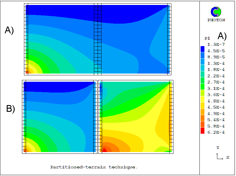
Transfer objects have 'surface' type and are placed always on the boundary of the computational domain. Part of the file created by library case 858 is reproduced below.
! (c) CHAM 2005 Exported from PHOENICS Version 3.6.0;  May 2005
! File name TROB1
! Transfer object
!
! Q1 commands
!
> OBJ, POSITION,  2.000000E-01,  0.000000E+00,  0.000000E+00
> OBJ, SIZE    ,  0.000000E+00,  2.000000E-01,  1.000000E+00
> OBJ, GEOMETRY,  default
> OBJ, ROTATION24, 1
> OBJ, TYPE, PLATE
! number of vertices
     8
! x, y, z of vertices
  0.0000E+00 0.0000E+00 0.0000E+00
  0.0000E+00 1.0000E+00 0.0000E+00
  1.0000E+00 1.0000E+00 0.0000E+00
  1.0000E+00 0.0000E+00 0.0000E+00
  0.0000E+00 0.0000E+00 1.0000E+00
  0.0000E+00 1.0000E+00 1.0000E+00
  1.0000E+00 1.0000E+00 1.0000E+00
  1.0000E+00 0.0000E+00 1.0000E+00
!
! number of facets
     6
! facet connectedness and colour
     1     2     3     4    80
     5     8     7     6    81
     1     4     8     5    80
     2     6     7     3    81
     4     3     7     8    82
     1     5     6     2    82
!
!-------------------data derived by In-Form
!
! number of cells in X, Y, Z direction
!      1    20     1
! X-coordinates of the cell faces
!  0.000000E+00
!  1.000000E-02
! Y-coordinates of the cell faces
!  0.000000E+00
!  1.000000E-02
  . . .
!  2.000000E-01
! Z-coordinates of the cell faces
!  0.000000E+00
!  1.000000E+00
! Field Values of P1
!  7.947696E-04
!  1.147313E-03
  . . .
!  6.130185E-04
! Field Values of U1
!  6.805007E-02
!  9.728204E-02
  . . .
!  9.946590E-02
! Field Values of V1
!  1.206840E-03
!  1.995379E-03
  . . .
!  0.000000E+00
! Field Values of H1
!  5.355338E-01
!  9.021159E-01
  . . .
!  1.000000E+00
! Field Values of C1
!  8.131076E-01
!  2.500963E-01
  . . .
!  8.074208E-12
It is the first part of the transfer-object file which corresponds
to that of the .POB file. Here such parameters are described
as a position, size of transfer object, number and coordinates
of vertices, number of facets, facet connectedness and colour.
In the second part, after 'data derived by In-Form', the parameters characteristic only for transfer objects are listed. Each new line begins with '!' symbol which is interpreted by Satellite as a beginning of the comment.
The numbers of cells in X, Y, Z direction are specified as integers after the appropriate comment.
Further the coordinates of cell faces are listed as reals consistently in X, Y, Z direction. The number of coordinates in each direction is equal to the number of cells plus 1.
Further the fields of all dependent variables follow as reals after the line 'Field Values of ...' where ... stands for the appropriate variable name.
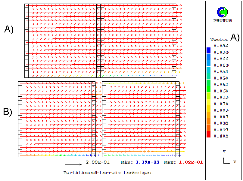
The field of the variable P1 contains the mass-flux values. The fields of other variables contain values of these variables near to the transfer-object surface. Number of values in each field equal the number of cells in the transfer object.
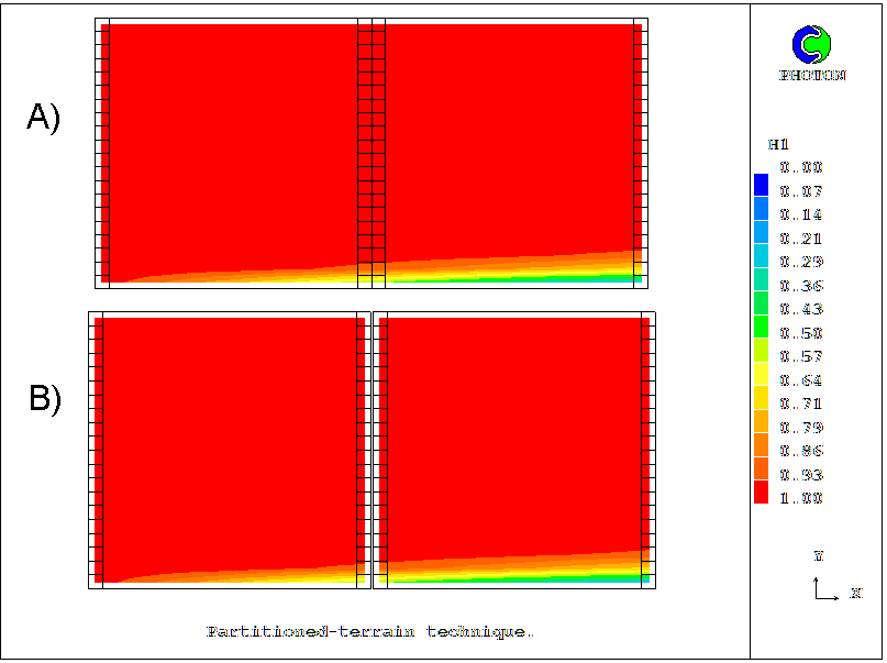
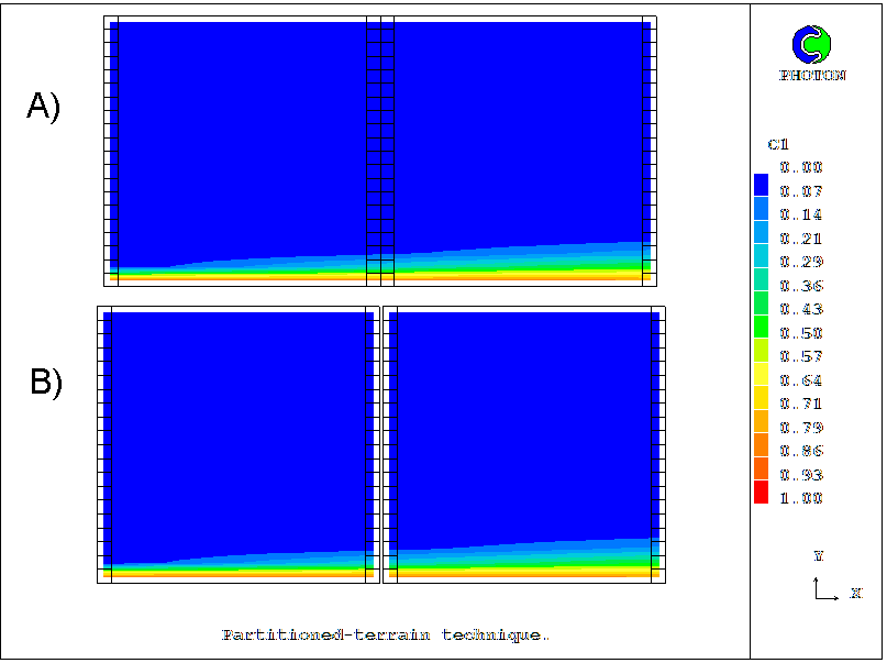
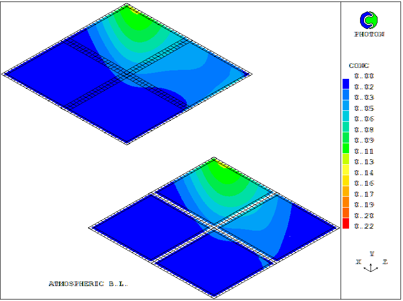
Input-file library case 855 concerns heat conduction in the z direction. The low wall is held at zero temperature while a fixed heat flux is applied at the right- hand end.
The grid, which extends also in the y-direction, is divided into two parts; but provision is made for the values of NY to differ in the two parts
                         !
        /----------------+-----------------/
   low  /                !                 / high
   wall /    1st part    !    2nd part     / wall
        /                !                 /
        / ---------------+-----------------/
              ^ y        !
              |-------> z-direction
The calculation for each part is executed in a separate run.Transfer object TROB1 for the high boundary is created at the end of the first run by means an In-Form (export statement.
The second run applies this information to its low boundary by reason of an In-Form (import' statements and then creates its own export object , TROB2 at its high boundary.
The area is divided into three parts as in the previous example.
                   !                 !
  /////////////////!// North Wall ///!///////////////////
  -----------------+-----------------+-------------------
 -->               !                 !                ->
 -->   1st run     !    2nd run      !    3rd run     -->
 -->C              !                 !                ->
  -----------------+-----------------+-------------------
  /////////////////!// South Wall ///!///////////////////
   ^ y             !                 !
   |-------> z-direction
TROB1 transfer object at high
boundary is formed at the end of the first run and is read
in the beginning of the second run. In a similar way, the data
are transmitted from the second run to third.
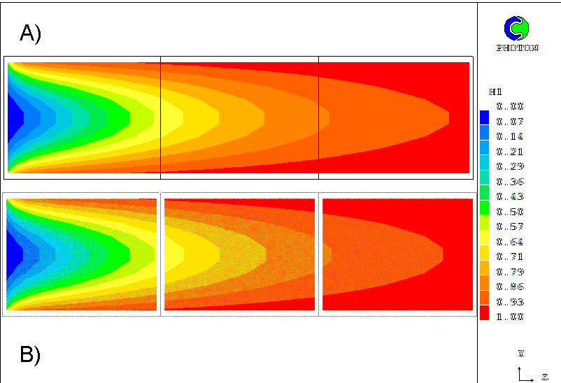
The fourth run simulates flow in the whole channel without the domain-partitioning technique for comparison with the previous runs.
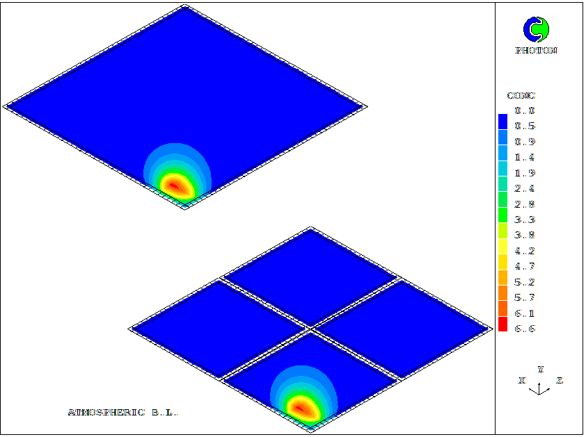
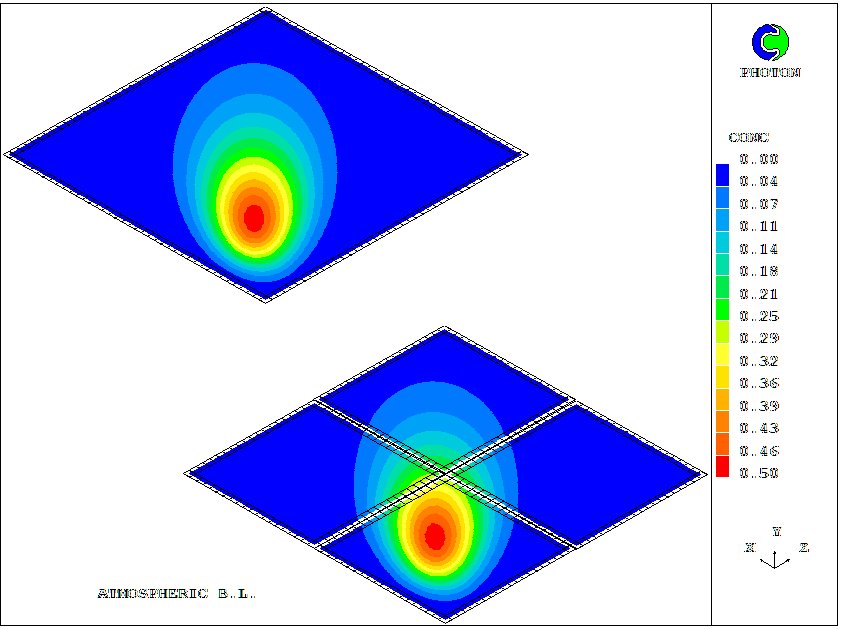
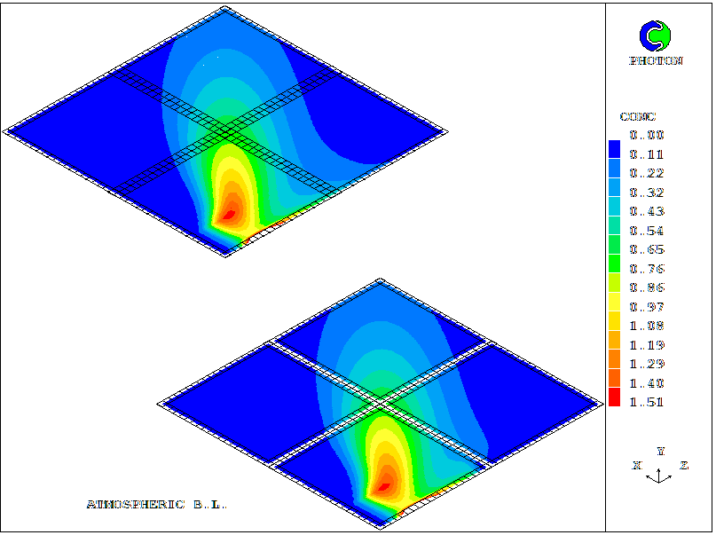
Comparison of results of calculations of the temperature and concentration
both with and without use of the domain-partitioning technique
are shown in the next pictures:
The values of variable h1 differ by a maximum of 6 %, while the values of c1 are identical.
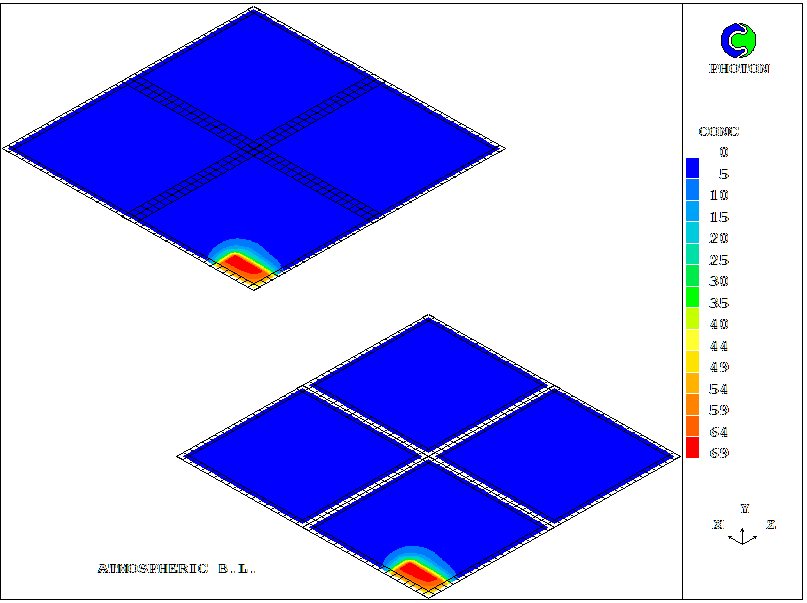
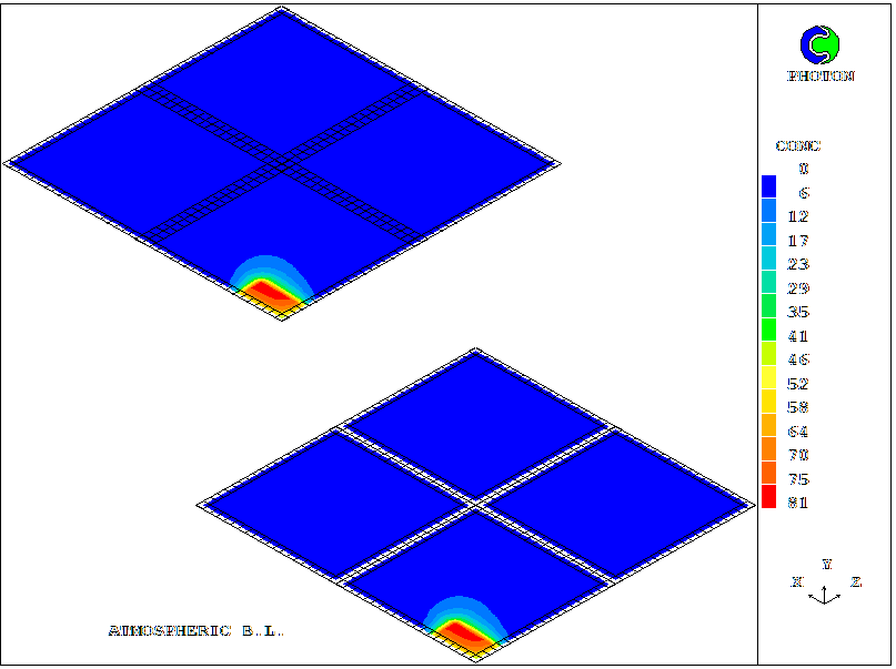
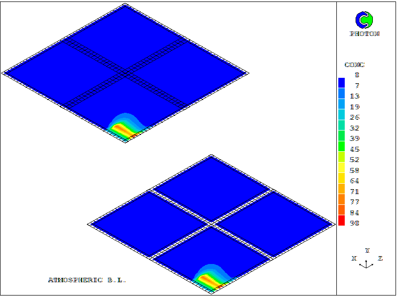
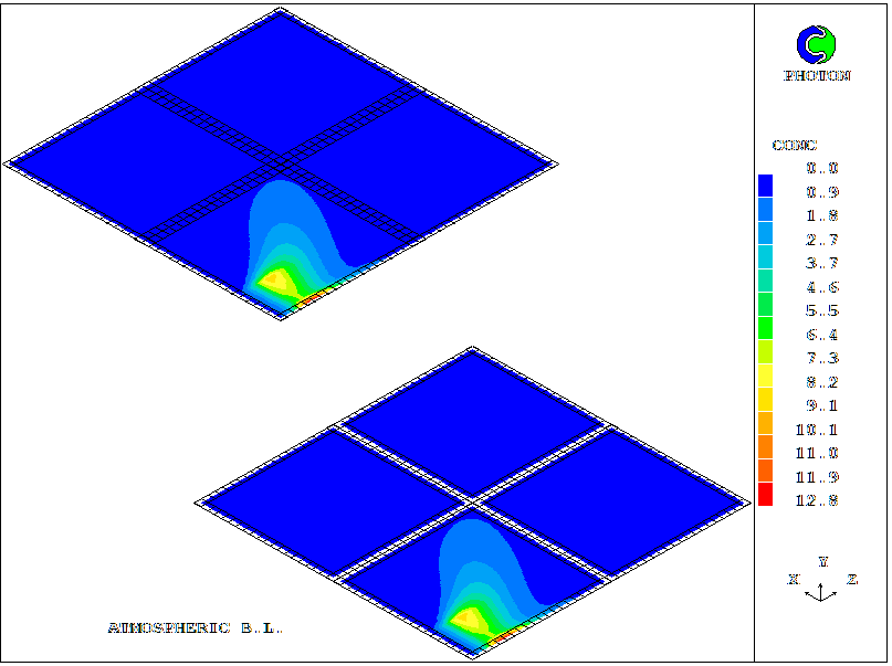
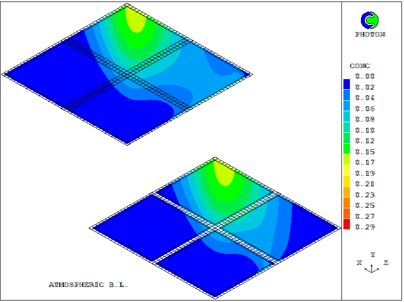
On the west side there is an inlet and on the north and east sides are outlets. The south side is a wall with constant temperature. In the south-west corner of the domain area there is a point source of pollutant..
The area is divided to two parts.
                      Outlet
               ---------------------
             I !         !         ! O
       U1    n !         !         ! u
       -->   l ! 1st run ! 2nd run ! t
             e !         !         ! l
        Y !  t !C        !         ! e
          !    --------------------- t
          !            Wall
          !----- X
The data are transmitted from the first run to second
by means of TROB1 transfer object
file.
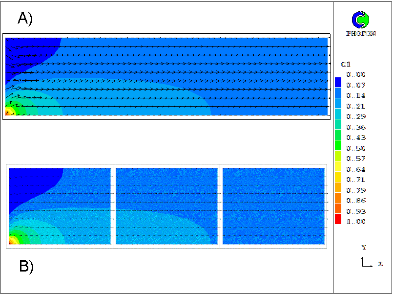
The third run simulate flow in whole area without the domain-partitioning technique for comparison with previous runs.
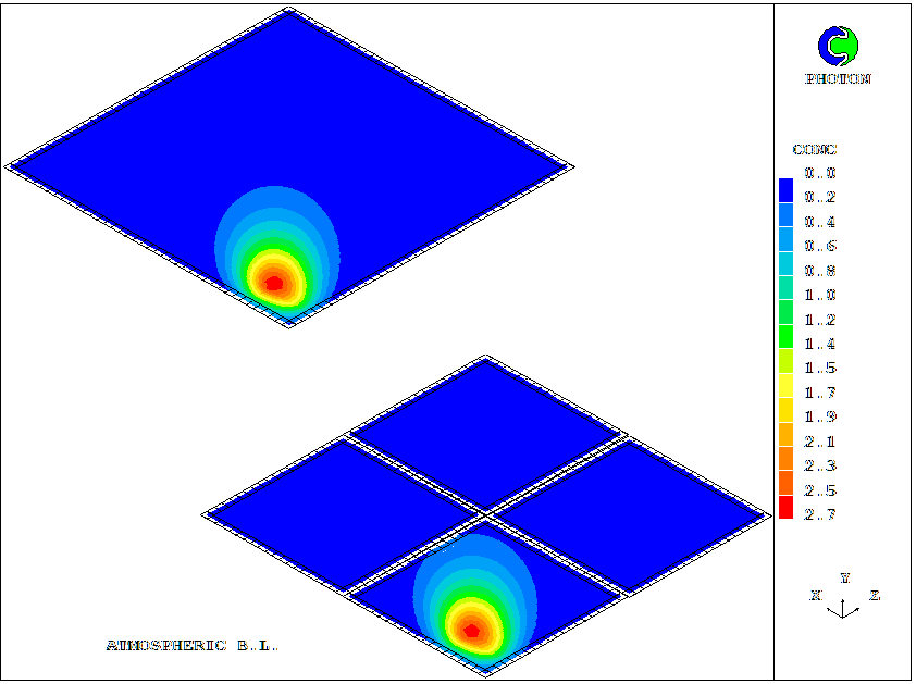
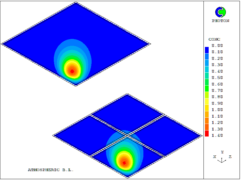
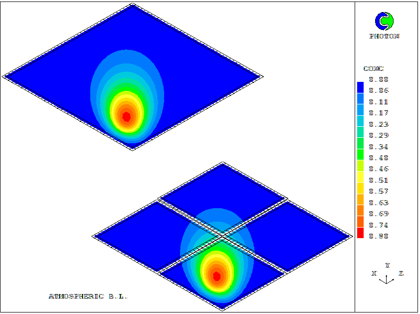
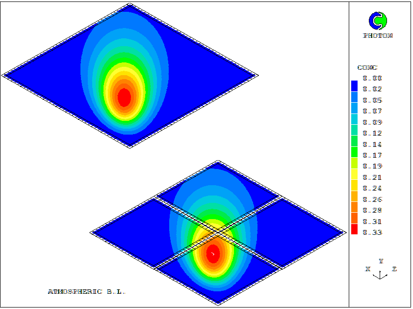
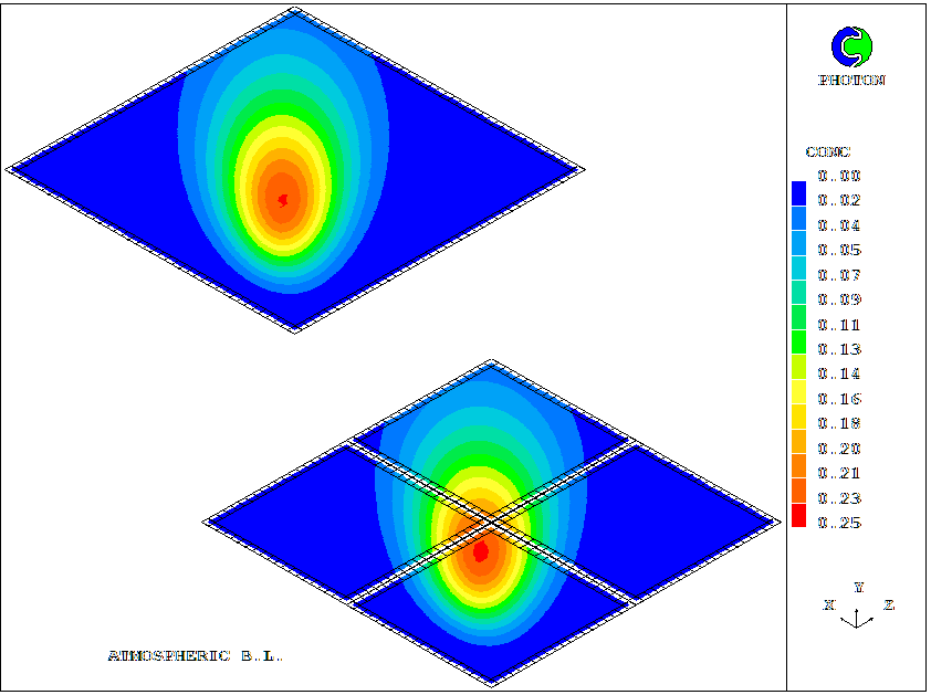
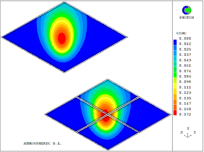
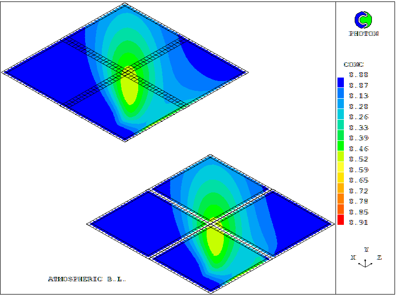
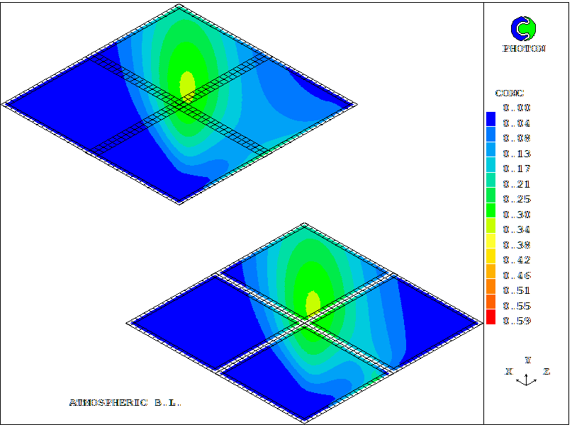
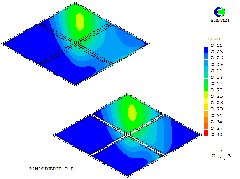
Comparison of results of calculations with a domain-partitioning technique and without it are shown in the next pictures :
 and
and
The values of variables h1 and c1 near the wall calculated in the second and third runs differ by respectively 3 and 2 %.
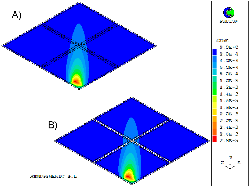
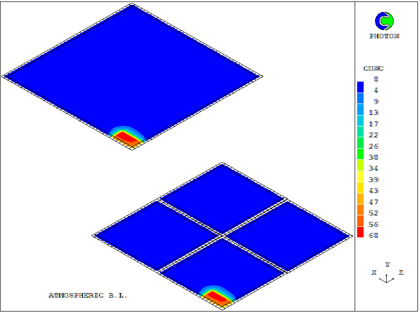
This example, which is case 858 of the core Input-File Library, explores distribution of pollutant over a large territory. Use of transfer objects permits to calculate uni-directional flow on small parts by one for other. The researched area according to the domain-partitioning technique in this case is divided on four parts as is submitted below.
HIGHTRO1 and EASTTRO1 transfer objects on high and east boundaries are formed at the end of the first run by means two '(export' In-Form statements. They store values of outlet mass flux and concentration on this boundaries for transfer them in second and third run.--------------------- ! ! ! ! ! ! ! 3rd run ! 4th run ! ! ! ! W1 ! ! ! --> ----------+---------- ! ! ! ! ! ! ! 1st run ! 2nd run ! ! ! ! X ! ! ! ! ! --------------------- ! ^ !----- Z /!\ ! !U1
The second run reads the information at low boundary from HIGHTRO1 object by means '(import' In-Form statements and at the end of calculations dumps it at east boundary in EASTTRO2 object.
The third run reads EASTTRO1 object and forms HIGHTRO3 object.
The fourth run reads the information from HIGHTRO3 and EASTTRO2 import transfer objects at low and west boundaries.
In general case the quantity of transfer objects can be any. Each run simulates distribution of pollution in an atmospheric boundary layer.
The wind profile at inlet boundaries is set by means of In-Form statements as a logarithmic velocity profile.
The ground relief (HIG variable) is calculated by In-Form formula.
MARK variable defined by In-Form is used for the image of ground relief in Photon.
The ground roughness are simulated by change of air density on height of a atmospheric layer. Density of air is calculated by barometric formula by means In-Form.
The fifth run simulates the flow in whole region
with the partitioning.
Its results are used for comparison with
Use of the domain-partitioning technique in unsteady calculations assumes the creation of transfer objects on each time step.
This case explores unsteady distribution of pollution at a large region of the ground.
The pollution source is set in the west-low corner and acts only at the first time step. Further the pollution cloud will be distributed by wind.
Use of the domain-partitioning technique similarly to the previous example. Except that the transfer objects are created and read at the each time step.
The positions of the spot at 500 second intervals are shown below:
 ,
,
 ,
, ,
,
 ,
, ,
,
 ,
, ,
,
 ,
,
This case simulates influences of value and direction of wind velocity on the position of pollution spot. The pollution source is set in the west-low corner and acts only at the first time step. Further the pollution cloud will be distributed by wind on a diagonal. But after NSTP time step the wind velocity increases and changes direction strictly at the left on the right.
The position of a spot after 500 second intervals are shown below:
Two further applications of the domain-partitioning technique will now be described.
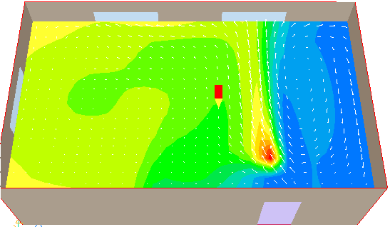
This simulation is represented by three q1 giles in the core input-file library. The first, case 860, simulates a fire in a living room. The resulting smoke escapes into a street through each window, as described by the TROBJ1, TROBJ2 and TROBJ3 export objects.
The second q1 file, case 861, simulates the distribution of smoke outside the building:
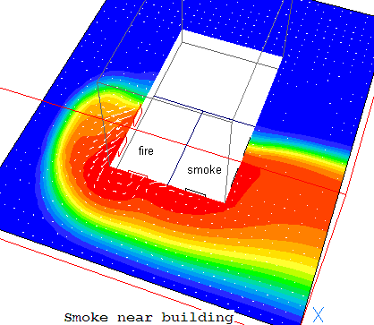
It then flows around the building and passes through the opened windows of an apartment neighbouring the first, being transferred via export objects connected with each window.
The third q1 file, case 863,
simulates the distribution of smoke inside this second apartment,
the concentrations of smoke entering through the open windows
being read from
import-object files. .
There follow the two corresponding q1 files created by VR Editor.
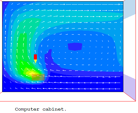
The first
simulates a convective heat exchange inside a computer cabinet
The second q1 file
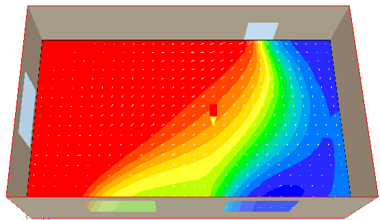
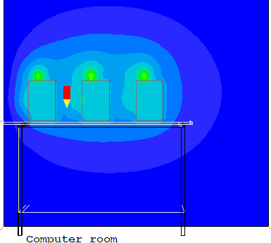
simulates heat exchange in the room.
The temperature values at all boundaries for each computer block
are read from transfer objects.
Strictly speaking, because the heated air leaving one of the computers can be drawn into the other, several iterations between the two scenarios should be made so as to investigate the importance of these effects.
It is most useful when the interaction between the partitioned domains is convective, and wholly from one domain to another; but with careful attention to detail, and sometimes a small amount of iteration, diffusive links can also be handled.
How to represent the pressure distribution at an outlet boundary to one domain and transmit it to another is also a matter which requires detailed study, in a case-by-case manner. All that will be stated here is that to postulate uniformity of pressure, although easiest to do, is seldom the optimal strategy.