ENC_Q1.HTM

Encyclopaedia Index click here for contents

Q1 file

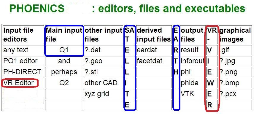
The Q1 file is an ASCII text file which the PHOENICS data-input module SATELLITE must read before it can do anything else, telling it first of all whether to operate in the batch or interactive mode, and then how many runs to make (see PHOENICS Encyclopaedia entry: RUN).

Its central position in the PHOENICS-module system is shown here:

The present article is therefore 'required reading' for the user of PHOENICS who wishes to master the mechanisms of data input.

The minimum Q1
The model Q1
A simple Q1 as an example
A historical review
How Q1 files are created
The parameterised Q1 (PQ1)

1. The minimum Q1

The minimum Q1 contains at least two lines, of which the first is typically:

TALK=T;RUN(1,1)

or:

TALK=F;RUN(1,1)

and the second is:

STOP

TALK=T tells SATELLITE to "converse" with the user, i.e. to start an interactive session.

TALK=F tells SATELLLITE not to converse, but simply to process whatever other commands it finds in the Q1, and then stop. (T and F mean TRUE and FALSE respectively in PIL).

RUN(1,1) instructs SATELLITE to stop at the first STOP line. (RUN(1,10) would mean: "Don't stop reading until you've reached the 10th STOP".

2. The model Q1

PHOENICS is supplied with model Q1, which resides in folder /phoenics/d_satell, as a reminder of what input data need typically to be introduced.
Its content is as follows:


TALK=T;RUN(1,1) 
    GROUP 1. Run title and other preliminaries 
    GROUP 2. Transience; time-step specification 
    GROUP 3. X-direction grid specification 
    GROUP 4. Y-direction grid specification 
    GROUP 5. Z-direction grid specification 
    GROUP 6. Body-fitted coordinates or grid distortion 
    GROUP 7. Variables stored, solved & named 
    GROUP 8. Terms (in differential equations) & devices 
    GROUP 9. Properties of the medium (or media) 
    GROUP 10. Inter-phase-transfer processes and properties 
    GROUP 11. Initialization of variable or porosity fields 
    GROUP 12. Patchwise adjustment of terms (in differential equations) 
    GROUP 13. Boundary conditions and special sources 
    GROUP 14. Downstream pressure for PARAB=.TRUE. 
    GROUP 15. Termination of sweeps 
    GROUP 16. Termination of iterations 
    GROUP 17. Under-relaxation devices 
    GROUP 18. Limits on variables or increments to them 
    GROUP 19. Data communicated by satellite to GROUND 
    GROUP 20. Preliminary print-out 
    GROUP 21. Print-out of variables 
    GROUP 22. Spot-value print-out 
    GROUP 23. Field print-out and plot control 
    GROUP 24. Dumps for restarts
STOP

The 24 lines between the first and the last are the names of the groups of data items which SATELLITE understands. (See GROUP, for systematically-arranged information about these.)

Because these lines start in the fifth column, they are treated by the Satelllite as comments which may be ignored; whereas TALK and STOP start in the first column and are therefore acted upon.

Some further rules about: blanks $, ! and +

SATELLITE responds only to statements on lines of which the first two characters are NOT blank, treating all others as comments.
So the T of TALK and the S of STOP must lie in column 1 or column 2 in order to take effect.

Six further points of note are:

Subsequent blanks are ignored, so that S T OP has the same effect as STOP.
Characters appearing after an exclamation mark are ignored.
Only the first 68 characters in a line are read by the satellite.
But inclusion of the dollar sign $ on or before the 68th character causes the next line to be read as a continuation of the first.
If a + sign appears in the first or second column, no matter how many blanks follow, it is interpreted as the instruction: "Do read this line." This allows indentation to be used so as to improve appearance,
Points 1. and 2. are not quite true of the In-Form statements which may appear in Q1 files; for unneeded blanks are not accceptable in In-Form statements; and ! has a special significance within them. These points are explained in the extensive In-Form documentation,

The lines which SATELLITE does take notice of are those which, as well as starting in one of the first two columns, are written in PIL, the PHOENICS Input Language.

3. A simple Q1 as an example

The richest source of Q1 files available to the user of Encylopaedia is the PHOENICS Input-File Library, which can best be inspected by clicking here.

Core-library case 116 will be chosen as a typical example, about which the following remarks can be made:

Clicking here will reveal that it starts with a large number of indented-two-spaces comments, namely those between the 'PHOTON USE' and 'ENDUSE' lines.
These are commands which, while being ignored by Satellite, are meaningful to the graphical-display packages PHOTON and VIEWER. They constitute a macro which it is useful to include in the Q1 file which generates the calculations, of which the macro is to display the results.
Clicking here reveals that, below the Group 1 heading, there appear not only the to-be read-by-Satellite TEXT and TITLE lines, but also many more two-spaces-indented ones, between the heading DISPLAY and the footer ENDDIS.
These are displayed on the screen in an interactive session so as to convey to the user what is the nature of the simulation.
GROUPS 4, 5 and 7 follow with PIL statements which set the grid in the y-z plane and determine which variables are to be solved and stored (the velocity potential) or only stored (the velocity components).
GROUP 11 contains an example ot the DO-loop structure which forms part of PIL; and it also illustrates the above-mentioned use of + in the first column.
There follow other Group entries on which there is no need to comment for present purposes.

4. A historical review

At this point it may be helpful to recount salient points of the history of the Q1 file, as follows, some information being drawn from the 'early-versions' file of the PHOENICS Chronicle:

When PHOENICS was first launched, in 1981, the Q1 did not exist. Instead, the problem-setting data were included as Fortran statements in the Satellite module, which did already exist separately from the equation-solving module, called Earth.
The Q1-file input procedure was initiated in 1984, as being, to paraphrase the above-linked document, 'more appropriate to PHOENICS than the then-fashionable menu-type input schemes of less-powerful software packages'.
Even if the reference to other packages (which were just beginning to compete) appears somewhat arrogant, those words do reflect a strand of thinking which still guides the development of PHOENICS: menus can never satisfy the needs of those users of PHOENICS who aspire to be innovative chefs rather than fast-food consumers.
CHAM strives still to make PHOENICS the CFD code of choice for ambitious innovators.
That does not imply that fast-food consumers were to be neglected. Indeed, having greatly enhanced the capabiliies of the PHOENICS Input Language during the intervening years, CHAM did provide for them, in 1989, its first menu-type data-input procedure.
This was indeed written in an interesting way (admittedly unseen by its users); for PIL was the language in which it was written,
In 1995, CHAM replaced the 1989 menu system with one which was more visually oriented, namely its 'Virtual-Reality' interface, the early history of which is recorded here. This did indeed make the input of data quick and easy; and it is the interface which the majority of PHOENICS users still employ.
Meanwhile, CHAM was also increasing the facilities which the 'ambitious chefs' could use by way of:
- PLANT (1997), which enabled them to insert formulae into the Q1 file which were then interpreted by the Satellite and converted into their Fortran equivalents so as to become, after computation and re-building, novel flow-simulation modules: and
- In-Form (2001), which enabled the same effect to be achieved without the Fortran-writing, compilation and re-building steps.
With hindsight, it can now be observed that the practices of the specialist ('chef') and majority ('consumer') users were allowed to diverge too far, in that the development of the Virtual-Reality Editor did not keep pace with the specialist advances. This delay, and its consequences, are discussed in the power-point presentation on Relational Data Input to PHOENICS.
This trend began to be reversed in 2007, with the introduction of the 'protected mode' of Satellite operation, whereby what was written in a Q1 file by a specialist user, was protected from being obliterated by the VR Editor.
At the present time (October 2008) therefore, increased attention is being paid to the creation of parameterised Q1 files, the nature of which will be discussed below.

5. How Q1 files are created

Acceptable lines in a Q1 file are usually introduced in one of five ways, listed here and explained in more detail immediately thereafter:

by the PHOENICS user, working outside PHOENICS with the aid of a text editor;
by the PHOENICS user, running the pre-processor (SATELLITE) in text mode, with TALK=T;
by the PHOENICS user, working in the same mode, and using the SATELLITE's own built-in EDITOR facility;
by SATELLITE itself, when the user has been working with it in "menu" or " VR-Editor" modes; or
by the PHOENICS pre-pre-processor, PRELUDE.

These will now be illustrated, as follows.

5.1 The use of a text editor

Let it be supposed that a user wishes to calculate the temperature in an electrically-heated steel slab, the faces of which at x=0 and x=0.1 m are held to zero degrees Celsius.
The heat-input rate per unit volume is 1.0 kW per cubic meter.
Then, knowing the elements of the PHOENICS Input Language, the user may write the following Q1 file:

TALK=T;RUN( 1, 1)
  DISPLAY
  Simulation of heat conduction in a steel slab of 0.1 m thickness,
  internallly heated by 1. kW/m**3 of electric power, with both its
  faces held to 0.0 deg Celsius
  ENDDIS
NX=100      ! Dividing the x dimension into 100 elements
XULAST=0.1  ! The thickness of the slab
GRDPWR(X,NX,XULAST,1.0) ! To create a uniform grid, namely one with
                        ! a power-law distribution, the exponent
                        ! being 1.0
SOLVE(TEM1) ! To solve for temperature
STORE(PRPS) ! To be able to set material properties via PROPS file
STORE(KOND) ! To be able to  print and check thermal conductivity
FIINIT(PRPS)=STEEL ! To require properties of steel to be used 
PATCH(minXface,WEST,1,1,1,1,1,1,1,1) ! To locate the low-x face
PATCH(maxXface,WEST,NX,NX,1,1,1,1,1,1) ! To locate the high-x face
COVAL(minXface,TEM1,FIXVAL,0.0)   ! To fix the values of both faces
COVAL(maxXface,TEM1,FIXVAL,0.0)   ! to zero
PATCH(HEATER,volume,1,nx,1,1,1,1,1,1)  ! To show that the volumetric
           ! heat flux extends from low x to high, i.e. from 1 to nx
COVAL(HEATER,TEM1,FIXFLU,1.e3) ! To fix the heat flux 1kW/m**3
STOP

These few lines are sufficient to enable:

the PHOENICS SATELLITE module, activated by the command RUNSAT, to read the Q1 and create an EARDAT file; and
the PHOENICS solver module, EARTH, activated by the command RUNEAR, to read the EARDAT file, to perform the computations, and print the RESULT file.

Here it should be explained, to those users who have not come across 'runsat', that it is not a PIL variable, and does not appear in the Q1 file. It is the name of one of the scripts (viz runsat.bat) used for running PHOENICS modules, the Encyclopaedia article on which can be seen by clicking here.
See also the relevant section of TR 326.
'Runear' is the name of another such script (runear.bat).

For those however who prefer to work via the PHOENICS SATELLITE module in interactive mode, it should be said that the same effect can be achieved by clicking 'run' at the top of the screen seen here:
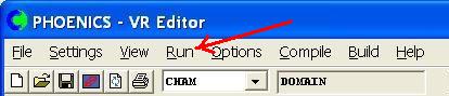
and then choosing 'pre-processor', 'text-mode (Satellite)' and Talk=F' from the successive drop-down menus.

The user needed to type only few lines because all PIL variables are supplied with 'default' values, which they retain unless the user sets new values. Thus the PIL variable LSWEEP, which specifies the last 'sweep' (i.e. outer iteration) which the solver should execute, is by default 1 .

The user was probably content to set no value for LSWEEP because he knew that, for this linear heat-conduction problem, a single sweep should suffice.

The computed temperature values in RESULT are as follows, in which it is seen that the values at only 5 x-locations are printed (because the user did not over-write the default print-control commands):

Field Values of TEM1
          2.500E-09   1.837E-02   2.744E-02   2.721E-02   1.767E-02
 IX=          1          21          41          61          81

Checking the correctness of the calculation

The value at the lowest-x plane in the slab, where IX=1, is indeed very close to the desired zero value; and elsewhere in the RESULT file can be found the line:

Nett source of TEM1 at patch named: HEATER   = 1.000001E+02

which, since the default dimensions of the domain in the y- and z-directions are both 1.0 m, corresponds to the specified heat input of 1 kW/m**3 . But are the other temperatures correct?

The user can answer this question by laboriously calculating by hand the ordinates of the parabolic temperature profile which represents the exact solution to the differential equation. But this is not necessary; for PHOENICS can be told to make the comparison itself.

This is done by introducing into the q1 file, the additional lines shown below in red:

SOLVE(TEM1) ! To solve for temperature
STORE(PRPS) ! To be able to set material properties via PROPS file
STORE(KOND) ! To be able to check the thermal conductivity
              ! To enable the correctness of the calculated values
              ! of temperature to be checked act, as follows:
CHAR(FORMULA) ! Declare the character variable FORMULA, and set it
              ! to the temperature calculated by PHOENICS, TEM1,
              ! divided by the theoretical temperature: namely, 
              ! thus:
FORMULA=TEM1/(0.5*1.E3*(XG-.005*:XULAST:)*(.995*:XULAST:-XG)/43.0)
              ! where
              ! 0.5 is a constant in the theoretical expression for
              ! the parabolic profile,
              ! 1.E3 is the volumetric heat input,
              ! xg = x value of any grid point,
              ! .005*:xulast: = xg of first grid point,
              ! .995*:xulast: = xg of last grid point,
              ! 43.0 is thermal conductivity of steel in PROPS file
(STORED var #RAT is :FORMULA:) ! Calculates the temperature ratio
(LONGNAME of #RAT print as tem1/theoretical_temperature)

These lines are designed to calculate and print the ratio of the temperature computed by PHOENICS to the analytically-derived temperature; and it is of course to be expected that the ratio is everywhere close to unity.

Only four of these lines are active, and therefore essential; the remainder are explanatory comments, introduced so as to bring to the attention of the present reader the existence of an easy-to-implement accuracy-checking feature, which makes use of the unique-to-PHOENICS In-Form facility.

The consequential RESULT file now contains the following new lines, in which it is seen that #RAT is indeed printed as unity everywhere except at IX=1. There, the very large departure from unity is without significance; it reflects the 2.5E-9 value of TEM1 computed there, divided by the even lower theoretical value, 0.0, to which 1.e-20 has been added to prevent a 'division-by-zero' Fortran error.

 Field Values of #RAT: tem1/theoretical_temperature
           2.500E+11   1.0         1.0         1.0         1.0
 IX=          1          21          41          61          81
 
 Field Values of KOND
 IY=   1   4.300E+01   4.300E+01   4.300E+01   4.300E+01   4.300E+01
 IX=          1          21          41          61          81
 
 Field Values of PRPS
           1.110E+02   1.110E+02   1.110E+02   1.110E+02   1.110E+02
 IX=          1          21          41          61          81
 
 Field Values of TEM1
           2.500E-09   1.837E-02   2.744E-02   2.721E-02   1.767E-02
 IX=          1          21          41          61          81

It can thus be concluded that the PHOENICS solution is indeed satisfactory.

Line-printer plots for speedy qualitative assessments

Another small addition to the Q1, namely:


 PATCH(TEM1PLOT,PROFIL,1,NX,1,1,1,1,1,1)
 COVAL(TEM1PLOT,TEM1,0.0,0.0)
 ORSIZ=0.2

enables the profile to be displayed by means of a line-printer plot, thus:


 PATCH(TEM1PLOT,PROFIL,   1, 100,   1,   1,   1,   1,     1,     1)
 PLOT(TEM1PLOT,TEM1, 0.000E+00, 0.000E+00)
   Variable    1 = TEM1
     Minval=  2.500E-09
     Maxval=  2.849E-02
     Cellav=  1.880E-02
 1.00 +....+....+....+....11111111111....+....+....+....+
 0.90 +               1111           1111               +
 0.80 +            111                   111            +
 0.70 +          11                         11          +
 0.60 +        11                             11        +
 0.50 +      11                                 11      +
 0.40 +    11                                     11    +
 0.30 +   11                                       11   +
 0.20 + 11                                           11 +
 0.10 +11                                             11+
 0.00 11...+....+....+....+....+....+....+....+....+...11
      0   .1   .2   .3   .4   .5   .6   .7   .8   .9  1.0
 the abscissa is       X  .  min= 5.00E-04 max= 9.95E-02

Such plots are not elegant; but, because they are so easily generated and often give the information which the user needs, they are not to be despised.

The use of declared variables

In the red lines above appeared the line:
CHAR(FORMULA) ! Declare the character variable FORMULA, and set it

PIL allows the declaration of new variables as characters, reals, integers and logicals. [It calls the latter 'booleans'.] The second of these is illustrated in the following modificaction of the first-shown Q1 file, in which the new features are again indicated by the red colour as follows:


TALK=F;RUN(1,1)
REAL(THICK,HEATINPT)  ! Declaration of new variables
THICK=1.0              ! Setting their values
HEATINPT=0.01   
NX=100      ! dividing the x dimension into 100 elements 
            ! the thickness of the block = THICK                 
GRDPWR(X,NX,THICK,1.0) ! to create a uniform grid, namely one with
                          a power-law distribution, the exponent 
                          being 1.0
SOLVE(TEM1) ! to solve for temperature
PATCH(minXface,WEST,1,1,1,1,1,1,1,1) ! to locate the low-x face                         
PATCH(maxXface,WEST,NX,NX,1,1,1,1,1,1) ! to locate the high-x face    
COVAL(minXface,TEM1,FIXVAL,0.0)   ! to fix the values of both faces                  
COVAL(maxXface,TEM1,FIXVAL,0.0)   ! to zero
PATCH(HEATER,volume,1,nx,1,1,1,1,1,1)  ! to show that the volumetric
                              ! heat flux extends from low x to high
COVAL(HEATER,TEM1,FIXFLU,HEATINPT) ! to fix the heat flux to HEATFLUX  
STOP

Here the parameters THICK and HEATINPT were introduced and set at the top of the file; and they were used lower down.

The computed results will of course of course be the same as before.

As will be seen below, the VR-Editor also treats the two q1s as identical; which (for reasons to be explained) is less desirable.

5.2 Text-mode interaction

If the user sets TALK=T in the first line of his Q1, the PHOENICS satellite responds to the command RUNSAT by presenting the screen shown here.

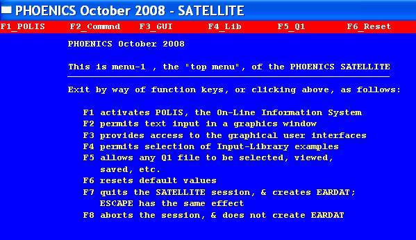
Pressing the F2 key leads to the next screen, which permits the interaction to begin:

The user can now make keyboard entries and read responses on the screen.

For example, if the user understands that the variable steel is recognised by the PHOENICS Satellite module as an integer and wishes to know its value, he may type 'steel' on the screen (case being unimportant) and will at once see:

Should the user then wish to to confirm that his selection of that material is conveyed to the solver by the setting of the value of the variable FIINIT(PRPS), entering 'fiinit(prps)' at the keyboard will elicit: :

Suppose now that the user wishes to replace steel by copper, first establishing which integer to use. Then entering 'copper' at the keyboard will reveal:

So as to make the change, the user should then type
'fiinit(prps)=copper' (or fiinit(prps)=103), and will see on the screen:

If the interactive session is now closed by pressing the F7 key, and the resulting Q1 file is inspected in any editor, it will be found that its last few lines are now as follows, showing that, as is true of all such interactions, new instructions are added to the bottom of the file:


FIINIT(PRPS)=STEEL ! To require properties of steel to be used
PATCH(minXface,WEST,1,1,1,1,1,1,1,1) ! to locate the low-x face
PATCH(maxXface,WEST,NX,NX,1,1,1,1,1,1) ! to locate the high-x face
COVAL(minXface,TEM1,FIXVAL,0.0)   ! to fix the values of both faces
COVAL(maxXface,TEM1,FIXVAL,0.0)   ! to zero
PATCH(HEATER,volume,1,nx,1,1,1,1,1,1)  ! to show that the volumetric
           ! heat flux extends from low x to high, i.e. from 1 to nx
COVAL(HEATER,TEM1,FIXFLU,1.e3) ! to fix the heat flux 1kW/m**3
FIINIT(PRPS)=COPPER
STOP

If now the solver is run, by way of the command RUNEAR, it will be found that the RESULT file now contains the lines:


Flow field at ITHYD=   1, IZ=   1, ISWEEP=     1, ISTEP=    1
 
 Field Values of KOND
           3.810E+02   3.810E+02   3.810E+02   3.810E+02   3.810E+02
 IX=          1          21          41          61          81
 
 Field Values of PRPS
           1.030E+02   1.030E+02   1.030E+02   1.030E+02   1.030E+02
 IX=          1          21          41          61          81
 
 Field Values of TEM1
           2.500E-09   2.073E-03   3.097E-03   3.071E-03   1.995E-03
 IX=          1          21          41          61          81

They show that the increase in thermal conductivity, to 381.0 from 43.0, has produced a proportionat reduction in temperature, as is to be expected (the heat input having been left unchanged).

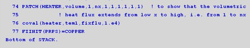
5.3 Use of the Satellite's built-in editor

Let us now suppose that the user wishes to increase the heat input ten-fold. He could do so during a text-interactive session by entering the line:


COVAL(HEATER,TEM1,FIXFLU,1.e4)

This line would then appear at the bottom of the screen; and, since Satellite reads and interprets lines in the Q1 from top to bottom, would over-ride the higher-up line.

However, invocation of the Satellite's built-in editor enables the higher-up line to be edited directly.

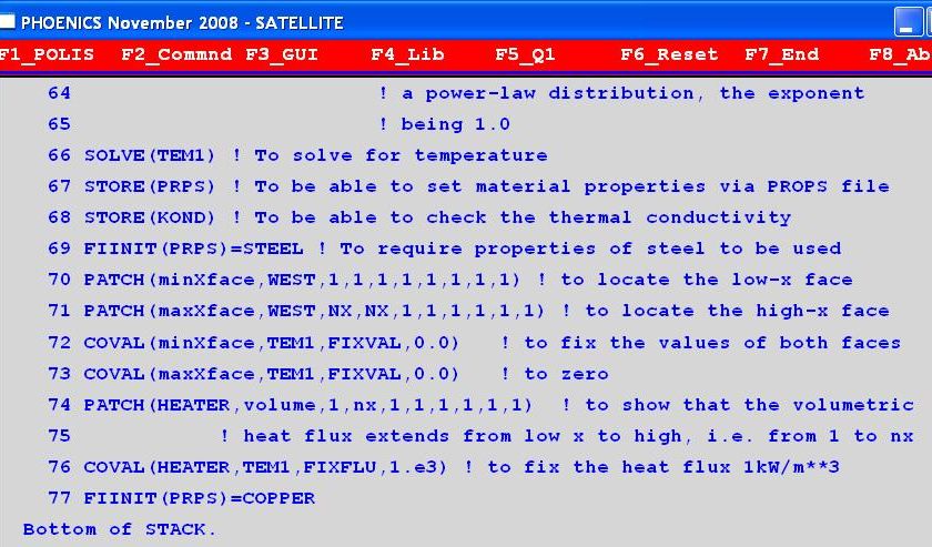
Thus, entering lb (meaning 'list from the bottom') in interactive mode elicits the screen shown here, Evidently the line to be changed is number 76.
The built-in editor has no 'replace' command; therefore the user must type d76 so as to delete the line, followed by:
i75
RETURN
COVAL(HEATER,TEM1,FIXFLU,1.e4)
RETURN
RETURN

Typing lb again will show that line 76 has indeed been replaced in the desired manner;

and, when the solver is run again, the temperatures will be found to have increased ten-fold as expected.

The built-in text editor is somewhat primitive, as has been admitted; but it has one advantage over a text editor: it edits not the q1 but the internal-to-satellite 'instruction stack'. It can therefore see, and allow the user to change, instructions which the satellite reads by default before it reads the Q1.

What these instructions are can be seen by issuing successively the commands: L1-15, L16-30, L30-45, etcetera so as to list them all, fifteen lines at a time.

The interested reader is free to study these; but no further comments will be made here.

5.4 Use of the VR-editor

The Virtual-Reality Editor is activated by, for example, issuing the command RUNVRE, wherein 'VRE' stands for 'Virtual Reality Editor'.

This editor is intended to assist users who are not conversant with PIL to write Q1 files for them; and indeed it does so. However, in the course of time, it has acquired the propensity to do much more.

Specifically, when supplied with a user-written Q1 file and nothing more, it re-writes it, in its own 'dialect' of PIL, with both advantages and disadvantages, some of which will now be discussed.

Let the Q1 which it reads be the first text-edited Q1 which was discussed above.

First it is instructive to look at the Q1 which the VR-Editor writes when it is simply opened and closed, without the user's having made any modification to the data whatsoever. It is shown here, with interspersed comments in brown font, explaining its differences, from the Q1 described above, with which the VR-Editor started.



TALK=T;RUN( 1, 1)
 
 ************************************************************
   Q1 created by VDI menu, Version 2008, Date 06/11/08
 CPVNAM=VDI;SPPNAM=Core

These are defaults of the VR-Editor (referred to as VRE from now on.)
SPPNAM=Core means that this is NOT a Special-Purpose Program.

For present purposes, there is no need to comment on every item. Readers who are interested in disregarded items, such as CPVNAM, can find explanations in the PHOENICS Encyclopaedia.


 ************************************************************
  Echo DISPLAY / USE settings
  DISPLAY
  Simulation of heat conduction in a steel slab of 0.1 m thickness,
  internallly heated by 1. kW/m**3 of electric power, with both its
  faces held to 0.0 deg Celsius
  ENDDIS
 ************************************************************
 IRUNN   =         1 ;LIBREF =         0
 ************************************************************
  Group 1. Run Title
 TEXT(No title has been set for this run.     )
 ************************************************************
  Group 2. Transience
 STEADY  =    T

The human editor knew that steady flow is the default, and therefore made no mention of the logical variable STEADY; but VRE is here seen to be more punctilious.



 ************************************************************
  Groups 3, 4, 5  Grid Information
    * Overall number of cells, RSET(M,NX,NY,NZ,tolerance)
 RSET(M,100,1,1,1.000000E-05)

This is an example of VRE's dialect of PIL.
The 100 is NX; the 1,1 are NY, NZ, the three integers being the numbers of intervals in the x, y and z directions, the defaults which the Human Editor (henceforth H.E.) did not need to mention. (1.000000E-05 is the default 'tolerance' which will not be explained here.)

It should be noted however that neither XULAST nor THICK appear, either explicitly or implicitly. VRE prefers numbers to characters.

It may also be noticed that VRE is not economical in its printing practices. We humans might find 1.E-5 sufficient; but VRE prints 1.000000E-05 .

 
 ************************************************************
  Group 6. Body-Fitted coordinates
 ************************************************************
  Group 7. Variables: STOREd,SOLVEd,NAMEd
 ONEPHS  =    T
    * Non-default variable names
 NAME(148) =KOND ; NAME(149) =PRPS
 NAME(150) =TEM1
    * Solved variables list
 SOLVE(TEM1)
    * Stored variables list
 STORE(PRPS,KOND)

H.E. did not need to say that this was a (default) one-phase phenomenon; and H.E. did not care into which member ot the NAME array TEM1 was placed.


 
 ************************************************************
  Group 8. Terms and Devices
 ************************************************************
  Group 9. Properties
    * Domain material index is 111 signifying:
    * STEEL at 27 deg c (C = 1%)
 SETPRPS(1,111)
 ENUT    = 0.000000E+00
 DRH1DP  = 5.000000E-12
 DVO1DT  = 3.700000E-06
 PRNDTL(TEM1) = -4.300000E+01

Here the VR-Editor has used the command
SETPRPS(1,111)
signifying "set the properties of the first-phase material to be those of the material with index number 111."
It is the equivalent of H.E,'s command:
fiinit(prps)-steel,
Both are legitimate PIL statements.

Once again, VRE uses the harder-to-read long form rather than the briefer equivalent:

 ENUT = 0.
 DRH1DP  = 5.E-12
 DVO1DT  = 3.7E-06
 PRNDTL(TEM1) = -4.3E+01

 
 
************************************************************
  Group 10.Inter-Phase Transfer Processes
 ************************************************************
  Group 11.Initialise Var/Porosity Fields
 FIINIT(KOND) =  1.001000E-10 ;FIINIT(PRPS) = -1.000000E+02
 FIINIT(TEM1) =  1.001000E-10
   No PATCHes used for this Group
 
 INIADD  =    F
  
  ************************************************************
  Group 12. Convection and diffusion adjustments
   No PATCHes used for this Group
 ************************************************************
  Group 13. Boundary and Special Sources
 
 PATCH (MINXFACE,WEST  ,1,0,0,0,0,0,1,1)
 COVAL (MINXFACE,TEM1, FIXVAL      , 0.000000E+00)
 
 PATCH (MAXXFACE,WEST  ,2,0,0,0,0,0,1,1)
 COVAL (MAXXFACE,TEM1, FIXVAL      , 0.000000E+00)
 
 PATCH (HEATER  ,VOLUME,0,0,0,0,0,0,1,1)
 COVAL (HEATER  ,TEM1, FIXFLU      , 1.000000E+03)

Here is something interesting: the indicial arguments of the PATCH command are different from those in the original Q1. This will be explained below.
The arguments of COVAL are the same however, albeit with a tiresome excess of spaces and zeroes.
There follow several groups in which both H.E. and VRE have tacitly adopted the default values.


  EGWF    =    T
 ************************************************************
  Group 14. Downstream Pressure For PARAB
 ************************************************************
  Group 15. Terminate Sweeps
 LSWEEP  =         1
 RESFAC  = 1.000000E-03
 ************************************************************
  Group 16. Terminate Iterations
 ************************************************************
  Group 17. Relaxation
 ************************************************************
  Group 18. Limits
 ************************************************************
  Group 19. EARTH Calls To GROUND Station
 ************************************************************
  Group 20. Preliminary Printout
 ************************************************************
  Group 21. Print-out of Variables
 ************************************************************
  Group 22. Monitor Print-Out
 NPRMON  =    100000
 NPRMNT  =         1
 ************************************************************
  Group 23.Field Print-Out and Plot Control
 NPRINT  =    100000
                              ISWPRF  =         1 ;ISWPRL =    100000
   No PATCHes used for this Group
 ************************************************************
  Group 24. Dumps For Restarts

Now begin some VRE-only settings. GVIEW has no counterpart in the original Q1, which was not concerned, as GVIEW is, with displaying the domain, grid and objects visually on the computer screen.

 
 
 GVIEW(P,0.000000E+00,1.000000E+00,0.000000E+00)
 GVIEW(UP,1.000000E+00,0.000000E+00,0.000000E+00)

> DOM,    SIZE,        1.000000E-01, 1.000000E+00, 1.000000E+00

The first 1.000000E+00 of SIZE ( of DOM, the domain) is the XULAST set by the user in his Q1, of which the 'block' occupies the whole of the domain. The other two are the default values of YVLAST and ZWLAST.

Of course, the line would be easier to inderstand, and equally acceptable to the SATELLITE, if it were printed as :


> DOM, SIZE, XULAST, YVLAST, ZWLAST


> DOM,    SCALE,       1.000000E+00, 1.000000E+00, 1.000000E+00
> DOM,    INCREMENT,   1.000000E-02, 1.000000E-02, 1.000000E-02
> GRID,   BOUNDS,       F F F F F F

> GRID,   RSET_X_1,     99, 1.000000E+00
> GRID,   RSET_X_2,      1, 1.000000E+00

Above is seen the way in which the VR-editor thinks of the 100-interval set by H.E., namely as 99 plus 1.
The reason is that the writer of the original Q1 file, probably through inadvertence, gave the patch on the east face the type 'west'. This made no difference to the solution, because the east and west areas of the cell have the same value; but the VR-Editor thought that it might have some significance.

 
> GRID,   RSET_Y_1,      1, 1.000000E+00
> GRID,   RSET_Z_1,      1, 1.000000E+00

Below it appears that the low-x and high-x patches which H.E. inserted have been converted into Virtual-Reality objects.
Their positions are now expressed in terms of real-number distances, instead of integer indices.

 
> OBJ,    NAME,        MINXFACE
> OBJ,    POSITION,    0.000000E+00, 0.000000E+00, 0.000000E+00
> OBJ,    SIZE,        0.000000E+00, 1.000000E+00, 1.000000E+00
> OBJ,    GEOMETRY,    default
> OBJ,    ROTATION24,        1
> OBJ,    TYPE,        USER_DEFINED
 
> OBJ,    NAME,        MAXXFACE
> OBJ,    POSITION,    9.900000E-02, 0.000000E+00, 0.000000E+00
> OBJ,    SIZE,        0.000000E+00, 1.000000E+00, 1.000000E+00
> OBJ,    GEOMETRY,    default
> OBJ,    ROTATION24,        1
> OBJ,    TYPE,        USER_DEFINED
STOP

without changing the relative geometrical positions of the physically-important physical features.

Nevertheless, it can be disconcerting; for, unless certain precautions are taken, the re-writing of the Q1 can involve loss of some important information which H.E. has supplied.

How this comes about is reported, at length, here.

Another example, case 116

Core-Input-Library case 116 was discussed above; and it exhibited the PIL-do-loop feature for setting porosities. It is interesting to observe what occurs when this Q1 is read into the VR-Editor.

The Q1 which the VR-editor creates as output, replacing and leaving no back-up of the one which it read, has no do-loop. Instead the implications of the initial do-loop are expressed thus:


 
> OBJ,    NAME,        HPOR1
> OBJ,    POSITION,    0.000000E+00, 0.000000E+00, 2.200000E+00
> OBJ,    SIZE,        1.000000E+00, 5.000000E-02, 3.400000E+00
> OBJ,    GEOMETRY,    cube14
> OBJ,    ROTATION24,        1
> OBJ,    TYPE,        BLOCKAGE
> OBJ,    MATERIAL,    199,Solid allowing fluid-slip at walls
 
> OBJ,    NAME,        HPOR2
> OBJ,    POSITION,    0.000000E+00, 5.000000E-02, 2.600000E+00
> OBJ,    SIZE,        1.000000E+00, 5.000000E-02, 2.600000E+00
> OBJ,    GEOMETRY,    cube14
> OBJ,    ROTATION24,        1
> OBJ,    TYPE,        BLOCKAGE
> OBJ,    MATERIAL,    199,Solid allowing fluid-slip at walls
 
> OBJ,    NAME,        HPOR3
> OBJ,    POSITION,    0.000000E+00, 1.000000E-01, 3.000000E+00
> OBJ,    SIZE,        1.000000E+00, 5.000000E-02, 1.800000E+00
> OBJ,    GEOMETRY,    cube14
> OBJ,    ROTATION24,        1
> OBJ,    TYPE,        BLOCKAGE
> OBJ,    MATERIAL,    199,Solid allowing fluid-slip at walls
 
> OBJ,    NAME,        HPOR4
> OBJ,    POSITION,    0.000000E+00, 1.500000E-01, 3.400000E+00
> OBJ,    SIZE,        1.000000E+00, 5.000001E-02, 9.999998E-01
> OBJ,    GEOMETRY,    cube14
> OBJ,    ROTATION24,        1
> OBJ,    TYPE,        BLOCKAGE
> OBJ,    MATERIAL,    199,Solid allowing fluid-slip at walls
 
> OBJ,    NAME,        HPOR5
> OBJ,    POSITION,    0.000000E+00, 2.000000E-01, 3.800000E+00
> OBJ,    SIZE,        1.000000E+00, 4.999997E-02, 1.999998E-01
> OBJ,    GEOMETRY,    cube14
> OBJ,    ROTATION24,        1
> OBJ,    TYPE,        BLOCKAGE
> OBJ,    MATERIAL,    199,Solid allowing fluid-slip at walls

These statements are very different in form from those of the original Q1; and indeed 'porosity' makes no appearance. Instead, the same fluid-flow-blocking effect achieved by the formerly-specified field of porosity is here effected by introduction of 'objects', to which the the Editor has automatically assigned the names HPOR1 etc.

Further, the positions of these objects are specified in terms of geometrical distances rather than by reference to grid indices. This has the advantage that they will retain their positions and sizes in space even though the fineness of the grid is increased.

However, how the porosity was at first defined has been lost sight of.

This loss is sometimes serious.

A source of further information

The above discussion has concentrated on the difference between the various 'dialects' of PIL which appear in differently-created Q1s.

A much fuller account of Q1s written by the VR-Editor can be found in the relevant section of TR326, accessed by clicking here.

5.5 Use of Prelude

The fifth means of Q1-writing involves use of the relatively new 'pre-pre-procesor' of PHOENICS, viz PRELUDE, the module in the diagram shown at the start of this article.
It is seen there that PRELUDE receives information from the 'gateway' shown on the left and passes it on, in the form of a Q1 file, to the Satellite.

Some extracts from such a Q1 now follow, together with some interpolated comments in brown font.

The flow scenario to which the Q1 relates is similar to that which will be discussed in section 6.1 below, namely that of the release of noxious gas into the atmosphere; and it will be seen that PRELUDE is able to write a 'parameterised Q1', the nature and merits of which are the subject of the whole of section 6.


TALK=T;RUN( 1, 1)
 
CPVNAM=VDI;SPPNAM=Core
 ************************************************************
    Group 1. Run Title 
 TEXT(case1)
  save1begin

PRELUDE uses the standard Group structure, and uses the save?begin and save?end protected-mode markers.

 
REAL(RELDIAM,RELANGL,WINDANGL,WINDVEL,GASPR,FLOORCO)
 REAL(MOLWT,WALLHIGH,SCALE,OUTDIST,INDIST,WALLTHCK)
 REAL(DOMWIDE,WALLDIST,DOMLONG,RELHIGH,PIPEZPOS,PIPEDIAM)
 CHAR(UWIND,TMODEL,GASDEN,GASVEL,GASFLO,PROFL)
 REAL(DOMHIGH)
 INTEGER(NZGRID,NYGRID,NXGRID)
 CHAR(VWIND,VPROFL,UPROFL)

PRELUDE starts by making declarations of variables (above) and then ascribing values to them (below)

 RELDIAM = .025 ! Leak diameter
 NZGRID = 35 ! number of Z cells
 RELANGL = 90. ! Gas-release angle (degrees)
 NYGRID = 30 ! number of Y cells
 WINDANGL = 0 ! angle (degrees) of wind relative to X axis
 NXGRID = 50 ! number of cells in X
 WINDVEL = 2 ! wind velocity at top of domain
 UWIND = :WINDVEL:*cos(:WINDANGL:*3.14159/180) ! U velocity of wind

The settings may be made by way of formulae (See above and below).
Each setting may carry an explanatory comment, after the exclamation mark.


 GASPR = 1.e5 ! pressure of gas above atmosphere
 TMODEL = ke ! Turbulence model
 FLOORCO = 0.005 ! friction coefficient on ground
 MOLWT = 28.9 ! Molecular weight of gas
 GASDEN = 1.189*:MOLWT:/28.9 ! gas density inferred from air
 GASVEL = (2*:GASPR:/:GASDEN:)^.5 ! gas velocity at escape
 GASFLO = :GASVEL:*:GASDEN:*:RELDIAM:^2*3.14159/4 ! mass of gas e$
scaping
 WALLHIGH = 2.5 ! Height of wall
 SCALE = :WALLHIGH: ! scale of objects
 OUTDIST = 14*:SCALE: ! distance downstream
 INDIST = 2.5*:SCALE: ! distance from start of domain to gas leak
 WALLTHCK = 0.2*:SCALE: ! thickness of wall
 DOMWIDE = 12*:SCALE: ! Width of domain
 WALLDIST = 7.5*:SCALE: ! distance from gas leak to wall
 DOMLONG = :INDIST:+:WALLDIST:+:OUTDIST: ! Length of domain
 RELHIGH = 0.4*:SCALE: ! Release height
 PIPEZPOS = 0.4*:SCALE: ! Position of gas leak above ground
 PIPEDIAM = 0.16*:SCALE: ! Pipe diameter
 DOMHIGH = 3.5*:SCALE: ! Height of domain
 PROFL = (zg/((:DOMHIGH:)))^(1./7) ! Profile of wind speed
 VWIND = -:WINDVEL:*sin(:WINDANGL:*3.14159/180) ! V velocity of w$
ind
 VPROFL = :VWIND:*:PROFL: ! Profile of Y velocity
 UPROFL = :UWIND:*:PROFL: ! Profile of X velocity
  save1end
 TEMP0 = 273.15 ! reference temperature (deg K)
 PRESS0 = 1.e5 ! reference pressure ( N/m**2)
 LSWEEP = 50 ! the last-sweep number
  save1begin
  Grid dimension rules
 REAL( NXCALC, NYCALC, NZCALC)
 NXCALC = :NXGRID:
 NYCALC = :NYGRID:
 NZCALC = :NZGRID:
  Domain size rules
 REAL( DOMXSZ, DOMYSZ, DOMZSZ)
 DOMXSZ = :DOMLONG:
 DOMYSZ = :DOMWIDE:
 DOMZSZ = :DOMHIGH:
  save1end
 CONWIZ= T
 ************************************************************
    GROUP 2 - Transience; time-step specification 
 ************************************************************
    GROUP 3. X-direction grid specification  
 INT( NXCE, NYCE, NZCE)
NXCE=NXCALC; NXCE
NYCE=NYCALC; NYCE
NZCE=NZCALC; NZCE
RSET(M,:NXCE:,:NYCE:,:NZCE:,0.03)
  save3begin
 nregX=5

 iregX = 1
 grdpwr(x,5,5.85,-1.15)
 iregX = 2
 grdpwr(x,10,2.4,-1.0)
 iregX = 3
 grdpwr(x,10,16.25,1.15)
 iregX = 4
 grdpwr(x,5,3.0,1.0)
 iregX = 5
 grdpwr(x,20,33.0,1.05)
  save3end

PRELUDE can set the computational grid, region-by-region

 
  save4begin
 nregY=1

 iregY = 1
 grdpwr(y,-30,30.0,0.9)
  save4end
  save5begin
 nregZ=2

 iregZ = 1
 grdpwr(z,25,4.375,1.0)
 iregZ = 2
 grdpwr(z,10,4.375,1.1)
  save5end
 ************************************************************
    GROUP 4. Y-direction grid specification   
 ************************************************************
    GROUP 5. Z-direction grid specification   
 ************************************************************
    GROUP 6. Body-fitted coordinates or grid distortion  
  save6begin
 nogrid= T
  save6end
 isg52=1
 ************************************************************
    GROUP 7. Variables stored, solved & named  
 STORE (u1)
 SOLUTN (u1, y, y, y, n, n, y)
 STORE (v1)
 SOLUTN (v1, y, y, y, n, n, y)
 STORE (w1)
 SOLUTN (w1, y, y, y, n, n, y)
 STORE (p1)
 SOLUTN (p1, y, y, y, n, n, y)

Prelude writes what-to-solve and what-to-store statements in a way which the Satellite can understand.

 
 STORE (gas)
 SOLUTN (gas, y, y, y, n, n, y)
 STORE (vabs)
 SOLUTN (vabs, y, n, n, n, n, y)
 STORE (mark)
 SOLUTN (mark, y, n, n, n, n, y)
 STORE (hhh)
 SOLUTN (hhh, y, n, n, n, n, y)
 STORE (den1)
 SOLUTN (den1, y, n, n, n, n, y)
 STORE (ke)
 SOLUTN (ke, y, y, n, n, n, y)
 STORE (ep)
 SOLUTN (ep, y, y, n, n, n, y)
 STORE (pg)
 SOLUTN (pg, y, n, n, n, n, y)
 ************************************************************
    GROUP 8. Terms (in differential equations) & devices 
 ************************************************************
    GROUP 9. Properties of the medium (or media) 
 PATCH(WHOLE,VOLUME,1,nx,1,ny,1,nz,1,lstep)
   using turbulence K-Epsilon
 TURMOD(KEMODL)
   properties inform statement derived from 0
  save9begin
   derived from props file 0: air
 (property den1 is 1.189+gas*(1.395-1.189))
   = 1.189 in props file

It can also write In-Form statements

 
 (property enul is 1.544e-005)
 (property cp1 is 1.4*8314.6/(28.9+gas*(34.08-28.9)*(1.4-1)))
   = 1005.0 in props file
  save9end
 ************************************************************
    GROUP 10. Inter-phase-transfer processes and properties  
 ************************************************************
    GROUP 11. Initialization of variable or porosity fields  
  save11begin
 (initial of u1 at whole is (:UPROFL:))
 (initial of v1 at whole is (:VPROFL:))
 (initial of gas at whole is (0.0))
(initial of MARK at ceiling is 1.3)
(initial of MARK at ceiling2 is 2.3)
(initial of MARK at floor is 4.3)
(initial of MARK at infob1 is 1 with infob_1)
(initial of MARK at infob2 is 2 with infob_2)
(initial of MARK at infob3 is 3 with infob_3)

and In-Form-object statements,

 
(initial of MARK at infob4 is 4 with infob_4)
(initial of MARK at infob5 is 5 with infob_5)
(initial of MARK at infob7 is 7 with infob_7)
(initial of MARK at infob8 is 8 with infob_8)
  save11end
 ************************************************************
    GROUP 12. Patchwise adjustment of terms (in differential equations) 
 ************************************************************
    GROUP 13. Boundary conditions and special sources 
  save13begin
  save13end
 PATCH(hhh,VOLUME,1,nx,1,ny,1,nz,1,lstep)
  save13begin
(stored of HHH at hhh is gas^.25)
   == ::Preludemw::case1.PATCH0 HIGH
PATCH(CEILING,HIGH,1,50,1,30,35,35,-1,-1)
(source of u1 at ceiling is coval(fixval,:UPROFL:) with fixv)
(source of v1 at ceiling is coval(fixval,:VPROFL:) with fixv)
   == ::Preludemw::case1.PATCH1 HIGH
PATCH(CEILING2,HIGH,1,50,1,30,35,35,-1,-1)
(source of w1 at ceiling2 is coval(1.e3,0.0) with fixv)
   == ::Preludemw::case1.PATCH2 LOW
PATCH(FLOOR,LOW,1,50,1,30,0,2,-1,-1)
(source of u1 at floor is coval(den1*vabs*:FLOORCO:,0.0) with fixv)
(source of v1 at floor is coval(den1*vabs*:FLOORCO:,0.0) with fix$
v!line)
 patch(infob1,west,1,nx,1,ny,1,nz,-1,-1)
(INFOB at infob1 is Box(0,0,0,1.2,30.0,8.75,0.0,0.0,0.0) with INF$
OB_1)
(source of w1 at infob1 is 0. with infob_1!fixv)
(source of p1 at infob1 is -1.e10*p1 with infob_1!line)
(source of u1 at infob1 is :UPROFL: with infob_1!fixv)
(source of v1 at infob1 is :VPROFL: with infob_1!fixv)

of various kinds.

 
 patch(infob2,east,1,nx,1,ny,1,nz,-1,-1)
(INFOB at infob2 is Box(((:DOMLONG:))-(1.2),0,0,1.2,30.0,8.75,0.0$
,0.0,0.0) with INFOB_2)

That is all that will be said about Q1s written by PRELUDE at the present stage; for it has enabled the major point to be made, namely that PRELUDE can handle features of the PHOENICS Input Language which the VR-Editor, as yet, can not.

It is therefore the pre-processor recommended to users who wish to employ 'parameterised Q1 files', the nature and advantages of which will now be described.

6. The parameterised Q1

6.1 An example

Core-library case 162 is a parameterised Q1 file. It will be discussed in some detail so as to explain, by way of example, what such a file consists of, and why and how it was created.

The situation in question can be seen below: a steady gas-release occurs into a space traversed by a cross-wind. Contours and an iso-surface are shown.

Parameterised Q1s (to be called PQ1s from now on) may be processed by the Satellite in 'silent mode', i.e. that in which no interaction with the user is allowed except by way of specially-provided statements. A convenient way of doing so is via the PHOENICS Commander's input file-library feature.

When case 162 is loaded in this way, the following image appears on the screen:

This lists some of the parameters of the situation being investigated. Inspection of the list suggests among other things that, unless the user decides otherwise:

the released gas is hydrogen sulphide (H2S);
the reference wind velocity is 2.0 meters per second, at an angle of 20 degrees;
the wind velocity varies with height (zG) in accordance with a one-seventh power law:
that the numbers of cells in the grid are 50, 30 and 35 in the x, y and z directions;
and so on.

There is no need, for present purposes, to study or explain all the entries in detail. It suffices to note that:

unlike the single-instance Q1s created by the VR-Editor, a PQ1 allows many different flow simulations to be conducted; and
the user may easily change the values of the key parameters without having to edit any file.

The PQ1 itself was written by means of a text editor, as will be seen; and its writer had to exercise a considerable amount of care, and indeed much more than the majority of users will be willing to exercise. This is therefore the point at which the distinction made in section 4, should be re-emphasised: PHOENICS caters for two classes of user, namely:

the specialist, referred to above as the 'innovative chef'; and
his customer, the 'consumer', whose task it is to make and flow simulations, but who should not be asked to create tools for himself.

It is the former who creates the PQ1; and it is the latter who reaps the benefit.

6.2 The appearance of the menu

It must now be admitted that the appearance of the menu is somewhat old-fashioned. This may be improved in the future; but, meanwhile a more modern appearance is provided if it is viewed via the VR-Editor graphical-user interface. This also has the advantage of enabling the domain, the objects within it, and the grid to be viewed.

If the user does prefer the VR-Editor, he or she must remember to act appropriately on exit; at which point the following image appears on the screen:

The wisest choice is then to remove the tick from the 'write-Q1' box, thus:

for otherwise, although all the important contents of the Q1 will be preserved, the Editor will have added some redundant lines of its own.

Are the changes made via the text menu saved into the Q1?

The answer to this question is: No. The changes will influence the next solver run which is made, because they have been transmitted to eardat; but they will not be reflected in the next run of the Satellite.

If more permanent changes to the Q1 are desired, they must be made via a text Editor, such as Notepad for example by opening the Q1 file for editing from the VR-Editor File menu.
Then, if it is desired to change the exponent of the prescribed wind-velocity profile, say, it is necessary to search for the line:

and then change the 7 to the desired number.

6.3 The structure of a PQ1

A typical PQ1 has the following structure:

A 'declarations' section in which the parameters of the case are declared as belonging to one or other of the four types of PIL variable, namely:
- real,
- integer,
- boolean (i.e. logical), or
- character;
a 'settings' section, in which values are provided for the declared variables, as well as for such standard PIL variables (which did not need to be declared) as are used as parameters of the problem.
The settings are of both direct and indirect kinds. For example, four real variables might be declared thus:
REAL(length,width,height,volume)
Then the following three direct settings might be made:
length=1.0; width=2.0; height=3.0
followed by one indirect setting, namely:
volume=length*width*height
an 'interactive section', which sends messages to the computer screen and provides opportunities for the user to modify some of the already-set parameters; and
a 'consequences' section in which more data are usually introduced, the attributes of which may be influenced by the above-set parameters.

All sections are protected by 'save' markers, as is appropriate to the use of the 'protected mode' of Satellite operation.

6.4 Example of a 'declarations' section

In the present and following sections, the PQ1 already referred to in section 6.1, Core-library case 162, will again be inspected in order that the most important features of PQ1-writing can be illustrated.

Its 'declarations' section can be seen by clicking here,

The data entries are organised according to type, i.e. real, integer, character or boolean; and each class is divided into:

'primary' parameters, which are those which are used for defining the problem, and which users might wish to alter interactively, and
'secondary' which are derived from the first or which are used as convenient intermediaries lower down in the Q1 file.

Thus, whereas domwide and domhigh are defined explicitly (n terms of SCALE), as will be seen, domlong, the domain length, is defined implcitly as being the sum of indist, walldist and outdist . Therefore the domain width and height are classed as 'primary' and the length as 'secondary'.

Similarly, setting the wind velocity and angle, windvel and windangl, enable uwind and vwind to be derived. Therefore the first pair are 'primary' and the second pair 'secondary'.

It should be understood that what is being described here is not what all users are forced to do but rather what one user decided to do. Although PIL does have rules which must be obeyed, it also allows its users great freedom.

6.5 Example of a 'settings' section

The 'settings' section of case 162 can be seen by clicking here,

The following remarks may assist understanding:

The user has organised his or her data-input statements more-or-less in the same order as that of the declarations; but there is no necessity for this.
What appear to be duplicate settings are not truly so; for lines starting with two spaces are inactive; and, if one active setting follows another, it is the last which is decisive.
The setting and subsequent use of the intermediate variable SCALE has presumably been introduced in order that, when the height of the wall, wallhigh is increased, all other linear dimensions increase proportionately.
Why the user wanted this to happen we need not inquire; and obviously, many variants of this practice could be envisaged.
This is a small example of the relational nature of the PHOENICS data-input procedures.
Why profl is declared as a character variable is now evident: it is used to define the formula according to the which the boundary velocity profiles must be computed.
It is used below in In-Form source statements; and In-Form always uses character strings for these.

6.6 Example of an 'interaction' section

The 'interaction' section of case 162 can be seen by clicking here,

The following remarks may assist understanding:

It has two main parts:
1. provision of informatiom about what inputs have been made so far, divided into five sections; and
2. question and answer about possible data changes; in which first the section number is requested where changes are to be made; and then opportunities are provided for changing individual parameters.
Part 1 makes use of the PIL mesg command, in which, in lines such as wall height=:wallhigh:, the colons mean: "print the value of what lies between them".
What then appears on the screen is:

whereafter obeying the instructions permits the desired changes to be introduced for the next run only.
[Click here for a reminder of what these last words mean.]
Part 2 is rather long; but its five-section structure is recognisable as corresponding to the five groups of data which appear in the just-seen image, each beginning with a PIL 'if' line such as:
```
 if(secno.eq.1) then  ! section number 1
```
and closing with an 'endif'. Here secno is one of the declared integer variables.
Part 2 would be even longer were it not for the use of four PIL subroutines named: CHREAL, CHINT, CHBOOL and CHCHAR.
It would be inappropriate to describe these in detail here; but interested readers can inspect them and, with the aid of Encylopaedia entries, elucidate their mechanism.
Clicking here will bring them into view.
Once again, readers are advised to recognise that the interaction section of case 162 is merely one person's idea of how a data-input menu should be constructed. Those who like it can copy it; and those who do not can use the available PIL commands in whatever different way suits them better.
PIL empowers; but it does not enforce.

6.7 Example of a 'consequences' section

The 'consequences' section of case 162 can be seen by clicking here,

The following remarks may assist understanding:

The entries associated with Group 1 of the Q1, i.e. those above 'save1end', are concerned with deriving the more important of the 'secondary' parameters from the values set for the 'primary' ones.
Thus the first few lines understandably set the molecular-weight parameter according to which of the five possible gases has been chosen.
Then the x- and y-direction velocity data are deduced from the windangl and profl parameters. And so on.
In Group3, concerned with setting the computational grid, it is seen that there are two situations envisaged.
1. The first, which is activated by setting the logical variable uniform true, provides the lines which make some settings directly and calls the macro unigrid for the remainder.
  The next lines of the Q1 file are then skipped as a consequence of the goto next, the label next being lower down in the file.
2. These next lines constitute the second grid-setting possibility, in which the grid is specified so as to have different finesses in different 'regions'.
Since the purpose of the present Encyclopaedia article is to explain the general features of parameterised Q1 files, but not to explain all details of case 162, only two further points regarding grids will be made at this juncture, namely:

Repeated use is made of variables such as xlen and nrx, which were declared earlier so as to serve as temporary holders of real and integer values; and
at the end of the whole grid-setting statement block, there appear the lines:

nogrid=t   ! setting needed to tell the Satellite not to modify
           ! the just-specified grid in any way

These lines are important; for, without them, the Satellite working in VR-Editor mode is always liable to modify the grid in order better to fit any VR-objects which are present.

There are several notable features of the boundary-condition (i.e. Group 13) settings in case162.

First, although being deactivated by having been moved out of the first and second columns, the do loop exemplifies use of an often-useful device viz the fixing of velocities (w1 in this case) to zero by means of a series of patches (in the 'COVAL statements of which the argument '1.E9' means 'fix very strongly', while the '0.0' means 'to zero').
The reason for doing so is not explained by any comment; but it might have been to determine why, when zero w1 was expected as the result of computation, that result was not being achieved.
Then fixing the velocity to what was expected, and learning (from the nett source print-out) what force was necessary to achieve it, can enable the nature of the disturbing influence to be detected.
Secondly, buoyancy is being represented by an In-Form source rather than by one of the difficult-to-remember GRDNx rules which date back to the early years of PHOENICS.
Thirdly the 'ceiling' patch, with horizontal velocities (u1 and v1) fixed to those of the wind, and vertical velocity (w1) allowed to settle itself so as to satisfy continuity, is a more plausible way of representing a 'sky' boundary than the often used 'impermeable-lid' condition.
Fourthly, extensive use is being made of In-Form objects of various kinds, namely:
- BOX objects for the open vertical-plane boundaries of the domain;
- another BOX object for the wall traversing the lower half of the domain;
- an (elongated) ELLIPSOID object for representing the pipe from which the gas release starts; and
- a POINT object for the release itself.
To focus on just the last-mentioned of these, the POINT object is introduced, and its attributes settled, by the following lines in the PQ1:
```
if(releas) then
io=io+1                             !  next infob, the gas release
mesg(at release, infob no is :io: gasflo=:gasflo:
patch(infob:io:,cell,1,nx/2,ny/4,3*ny/4+1,1,nz/2,1,1)
(infob at infob:io: is point(:indist:,:domwide/2:,:pipezpos+pipedi$
am/2:,0.01) with infob_:io:)
(source of p1 at infob:io: is :gasflo: with infob_:io:)
(source of u1 at infob:io: is :gasvel:*:cos(relangl): with infob_:i$
o:!only)
(source of w1 at infob:io: is :gasvel:*:sin(relangl): with infob_:i$
o:!only)
(source of gas at infob:io: is 1.0 with infob_:io:!only)
endif
```
Among the parameters to be seen here are, as is understandable, are:
- gasflo, the flow rate of released gas, in kg/s,
- gasvel, the gas velocity, in m/s, and
- relangl, the release angle in radians.
Why the expressions are precisely as they are can learned by studying the relevant documentation, which it would however be inappropriate to summarize here.

6.8 Tutorials

Users of PHOENICS who wish to learn how to create PQ1s for themselves are advised to study the series of tutorials which is being prepared. This includes at the time of writing (April 2009):

PQ1-tutorial 1 Part 1, which comments upon core-library case 163, a PQ1 containing, in one file, the Q1s introduced in section 5.1 above;
PQ1-tutorial 1 Part 2, which explains how to extend the simulation capabilities of case 163, and how to introduce more user interactivity.
PQ1-tutorial 2 Part 1 and Part 2, , which show how to parameterize a pre-existing non-parameterized Q1, namely core library case 621, which itself is the outcome of a much-earlier tutorial, concerned with flow through a two-dimensional labyrinth.

Q1 file

Contents

1. The minimum Q1

2. The model Q1

Some further rules about: blanks $, ! and +

3. A simple Q1 as an example

4. A historical review

5. How Q1 files are created

5.1 The use of a text editor

Checking the correctness of the calculation

Line-printer plots for speedy qualitative assessments

The use of declared variables

5.2 Text-mode interaction

5.3 Use of the Satellite's built-in editor

5.4 Use of the VR-editor

Another example, case 116

A source of further information

5.5 Use of Prelude

6. The parameterised Q1

6.1 An example

6.2 The appearance of the menu

Are the changes made via the text menu saved into the Q1?

6.3 The structure of a PQ1

6.4 Example of a 'declarations' section

6.5 Example of a 'settings' section

6.6 Example of an 'interaction' section

6.7 Example of a 'consequences' section

6.8 Tutorials