Simultaneous Prediction of Solid stress, Heat transfer and
Fluid flow by a Single Algorithm
By Brian Spalding
Lecture presented at XIII School-Seminar of Young Scientists and
Specialists under the leadership of the Academician, Professor A.I.Leontiev
May 20-25, 2001, Saint Petersburg, Russia
next or contents
Abstract
- It is often believed that FLUID-FLOW and SOLID-STRESS problems
MUST
be solved by DIFFERENT methods and DIFFERENT computer programs.
- This is NOT TRUE, if the solid-stress problems are formulated in terms
of DISPLACEMENTS.
- The lecture exemplifies and explains how both DISPLACEMENTS and
VELOCITIES can be calculated AT THE SAME TIME.
- ALSO described, incidentally, are economical methods of simulating:
- thermal RADIATION between solids immersed in fluids; and
- TURBULENT CONVECTION at low Reynolds numbers in the same situation.
next or back
Contents
- The problem
- Its essential nature
- Practical occurrence
- The conventional solution
- A better solution
- A multi-physics example
- Stresses resulting from radiation, conduction and
convection
- Vector and contour plots
- How the stress calculations were performed
next or back or
contents
- The mathematics of the method
- Similarities between the equations for displacement and velocity
- Deduction of the associated stresses and strains
- The "SIMPLE" algorithm for the computation
of displacements
-
More details of the equations
- Details of the auxiliary models
- IMMERSOL, for radiation
- WGAP, WDIS and LTLS, for radiation and turbulence
- LVEL, for turbulence
- Conclusions
- References
next or back or
contents
1. The problem
(a) Its essential nature
It is frequently required to simulate fluid-flow and heat-transfer
processes in and around solids which are, partly as a consequence of the
flow, subject to thermal and mechanical stresses.
Often, indeed, it is the stresses which are of major concern, while
the fluid and heat flows are of only secondary interest.
next, back or contents
(b) Practical occurrence
Engineering examples of fluid/heat/stress interactions include:
- gas-turbine blades under transient conditions;
- "residual stresses" resulting from casting or welding;
- thermal stresses in
nuclear reactors during emergency shut-down;
- manufacture of bricks and ceramics;
- stresses in the cylinder blocks of diesel engines;
- the failure of steel-frame buildings during fires.
next, back or contents
(c) The conventional solution
It has been customary for two computer codes to be used for
the solution of such problems, one for
the fluid flow and the other for the stresses
Iterative interaction between the two codes is then employed, often
with considerable inconvenience.
next, back or contents
(d) A better solution
It is however possible for fluid flow, heat flow and
solid deformation, and the interactions between them, all to be
calculated at the same time.
The method of doing so exploits the similarity between the
equations governing velocity (in fluids) and those governing
displacement (in solids).
In the present lecture, the results of such a calculation
will be shown first.
The explanation of how it was conducted will then follow.
next, back or contents
2. A multi-physics example
(a) Description:
The task is to calculate the stresses in radiation-heated
solids cooled by air.
    20 deg C| air
            |             80 deg C
          | V |/////// hot radiating wall ///////////|
          |   ----------------------------------------
          |                       duct              ----->  exit
          |-------------                 -------------
          |// steel ///|     cavity      |/// steel /|
          |------------------------------------------- ? temperature ?
          |////////////// aluminium /////////////////|
          |-------------------------------------------
next, back or contents
Details of the calculation are:
- The Reynolds number (based on the inflow velocity and horizontal duct
width) is 1000.
Therefore the
LVEL model
is used for simulation of the
turbulence.
- The radiative heat transfer is represented by the
conduction-type
IMMERSOL model,
which is:
- economical and
- fairly accurate
for such situations.
The absorptivity of the air is taken as 0.01 per meter;
the scattering coefficient as 0.0;
and the solid surface emissivity as 0.9 .
next, back or contents
- Both LVEL and IMMERSOL make use of the distributions of:
- distance from
the wall (WDIS) and
- distance between walls (WGAP), both of which are
calculated by solving a scalar equation for the
- LTLS variable.
- The stresses within the metals result primarily from the differences in their
thermal-expansion coefficients. namely:
- 2.35 e-5 for aluminium, and
- 0.37 e-5 for steel.
next, back or contents
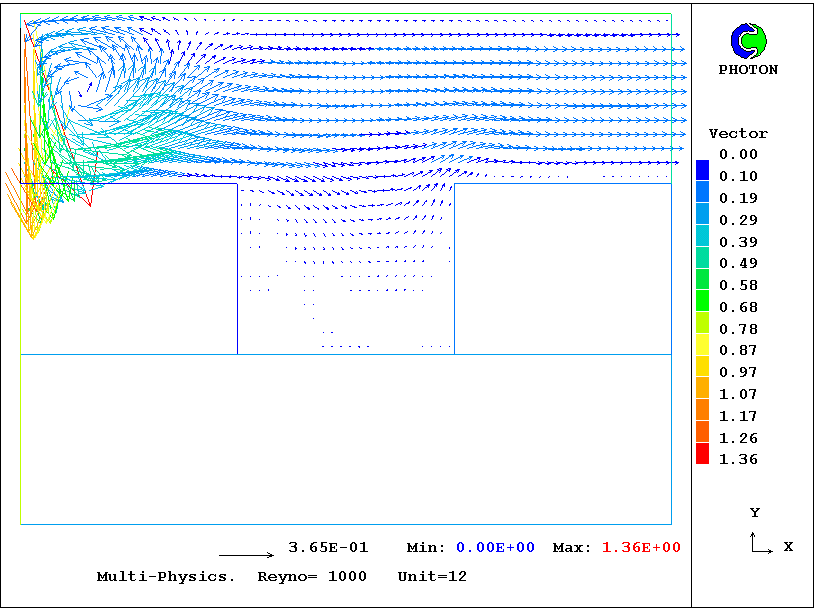
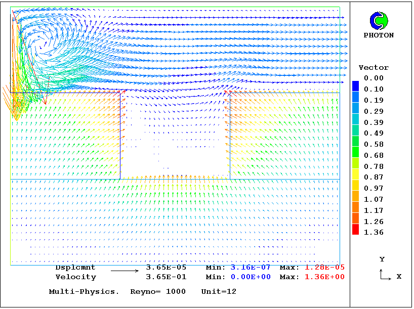
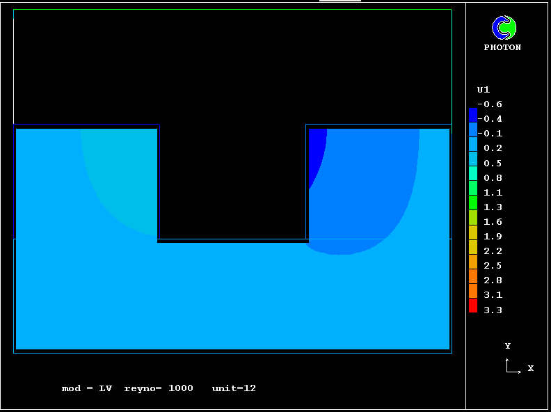
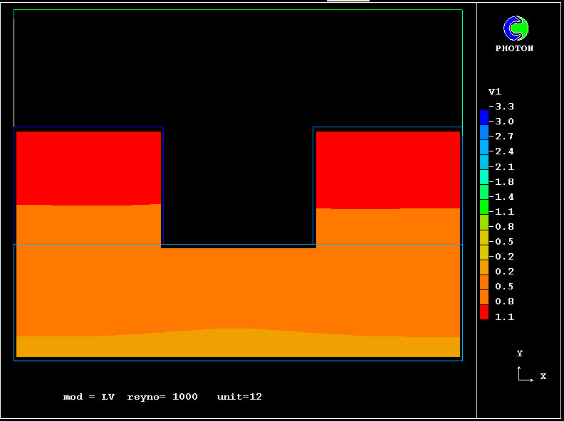
(b) Vector and contour plots
Vectors
The velocity vectors displayed in
Fig.1 reveal the
nature of the air-flow pattern.
They are calculated at the same time as the displacement vectors shown
additionally
fig.2;
but, of course, the two sets of vectors have different scales, and indeed
dimensions.
next, back or contents
The solids are supposed to be confined by a stiff-walled box, but are
allowed to slide relative to its walls. This is why the displacement
vectors are vertical near the confining-box walls.
They are however not allowed to slide relative to each other; this is
what causes the concentrations of stress at their contact surfaces.
next, back or contents
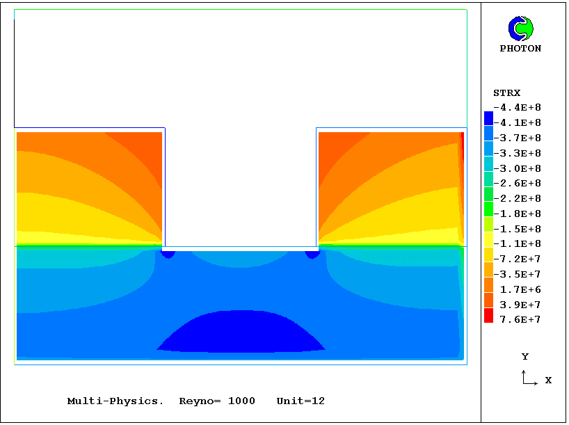
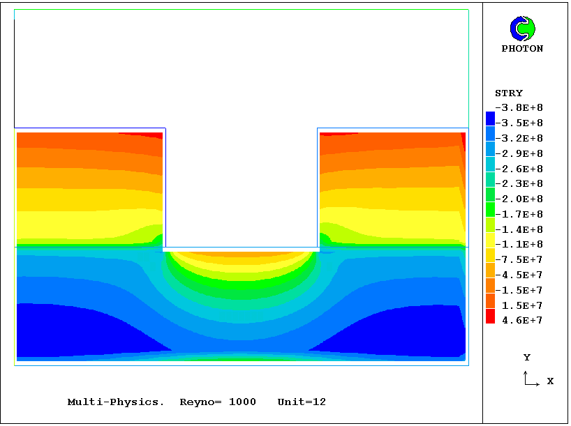
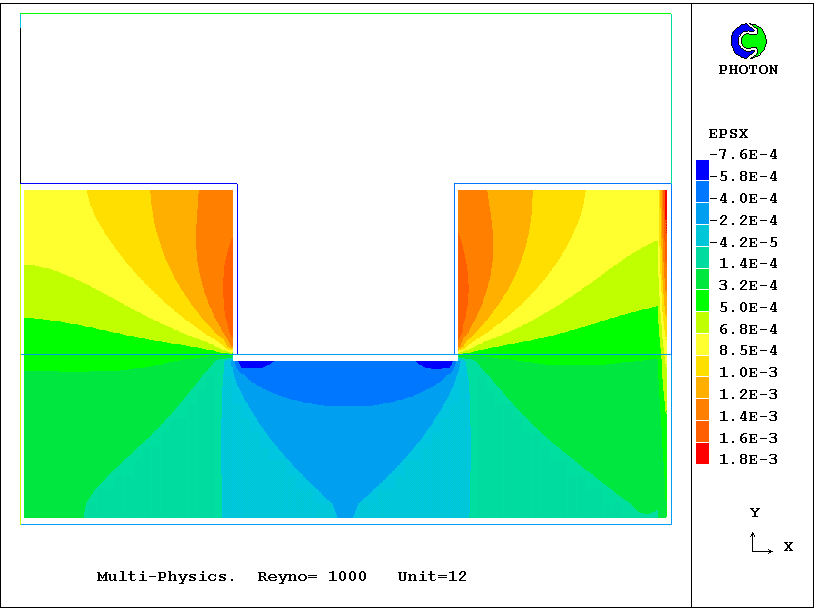
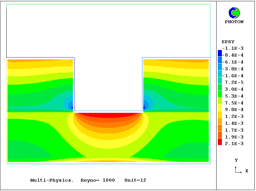
- Stresses and strains
The stresses in the x- (horizontal) and y- (vertical) directions are
displayed in
Fig.3 and
Fig.4
respectively.
They have been deduced from the strains shown in
Fig.5 for the x-direction , and in
Fig.6 for the y-direction,
next, back or contents
The strains have been deduced from the displacements by
differentiation.
The displacements, which were already shown as vectors in
Fig.2,
are displayed via contour plots :in
Fig. 7 for the x-direction
and
Fig. 8 for the y-direction.
It is from their (small) variations that the stresses and strains
are computed; but, these being small, their representations by way
of contours are not dramatic visually.
That is the end of the stress-strain results.
Now will be
shown some of the other variables which had to be computed.
next, back or contents
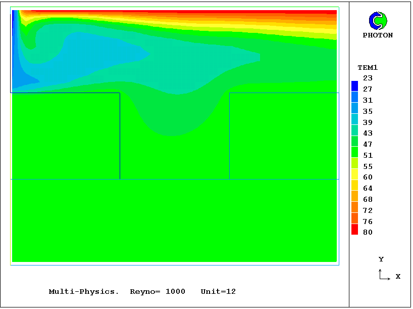
- Temperature fields
Fig. 9 displays contours
of temperature in the air and the solid, and reveals that:
- the air is heated by contact with:
- the 80-degree-Celsius top wall, and
- the metal blocks, which have been receiving heat by radiation
from the top wall;
- temperature differences within the high-conductivity solids are too small
to be discerned visually.
next, back or contents
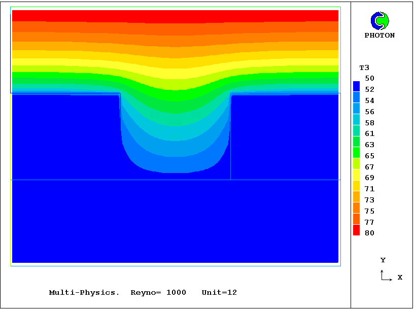
It is interesting to compare Fig. 9 with
Fig. 10.
This displays
the distribution within the air space of:
- the "radiation temperature", T3, which:
- is computed by IMMERSOL, and
- is defined as the temperature which would be taken up
by a probe which was affected only
by radiation.
Obviously, and understandably, T3 and TEM1 have very different
values, unless the absorptivity is very great (as in solids).
next, back or contents
The solid temperature influences the stresses and strains, of course,
primarily through the agency of the temperature-dependent
thermal-expansion distribution.
However, its variations with position, within a single material, are too
slight to be revealed by a contour diagram, as inspection of
Fig. 11 will reveal.
next, back or
contents
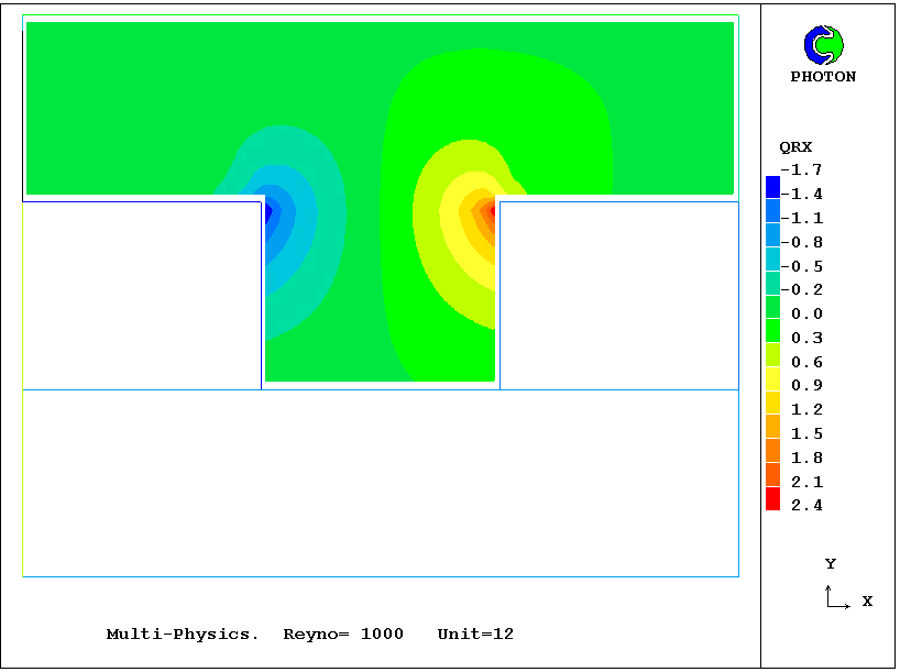
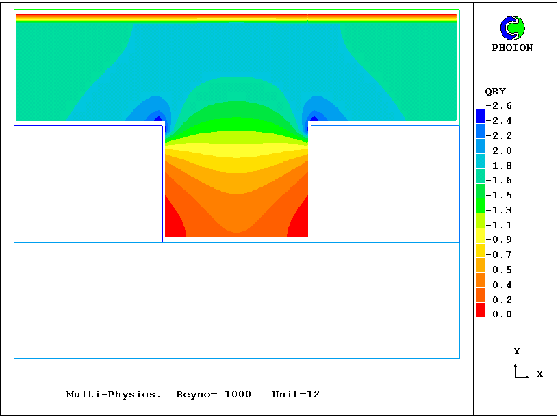
- Radiation-flux contours
The IMMERSOL model, of which the solution of the T3 equation is the
major feature, enables the radiant heat fluxes in the coordinate
directions to be established by post-processing.
The results are displayed in
Fig. 12 for the
x-direction. and by
Fig. 13 for the
y-direction.
The values and patterns displayed, if studied and interpreted in physical
terms, will be found to be plausible.
Where calculation by hand is easy, namely for the parallel surfaces,
they will be found to be correct.
next, back or
contents
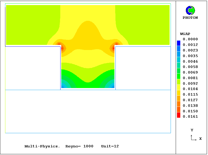
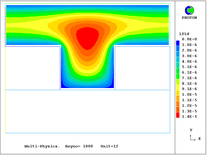
- Contours of auxiliary quantities used by IMMERSOL
A crucial feature of the IMMERSOL model is its use of the distribution of
the "distance between the walls", WGAP.
This quantity, which has an
easily-understood meaning when the walls are near, and nearly parallel, is
computed from the solution of the "LTLS" equation;
this will be explained later in the lecture.
The distributions of these two quantities are shown by
Fig. 14
for the former, and by
Fig. 15
for the latter.
next, back or
contents
It will be seen that WGAP has a uniform value in the region of
between the top of the duct and the tops of the upper metal slabs,
between which the actual distance is 0.008 meters.
Further, it has approximately twice this value near the convex
corners; and it becomes zero in the concave corners.
next, back or
contents
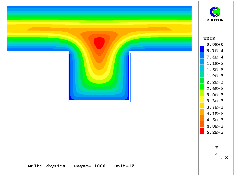
- Contours of auxiliary quantities used in the fluid-flow
calculation
The flow field was calculated by means of the LVEL turbulence
model,
which makes use of the wall-distance (WDIS) field.
This, like WGAP, is also
derived from the LTLS distribution.
The contours of WDIS are displayed in
Fig. 16.
which exhibits:
- the expected maximum of 0.004 between the parallel
horizontal walls, and
- a somewhat greater value near the cavity,
where the true distance from the wall depends on the direction in
which it is measured.
next, back or
contents
LVEL, like IMMERSOL, is a "heuristic" model, by which is meant that
it is incapable of rigorous justification, but is nonetheless
useful.
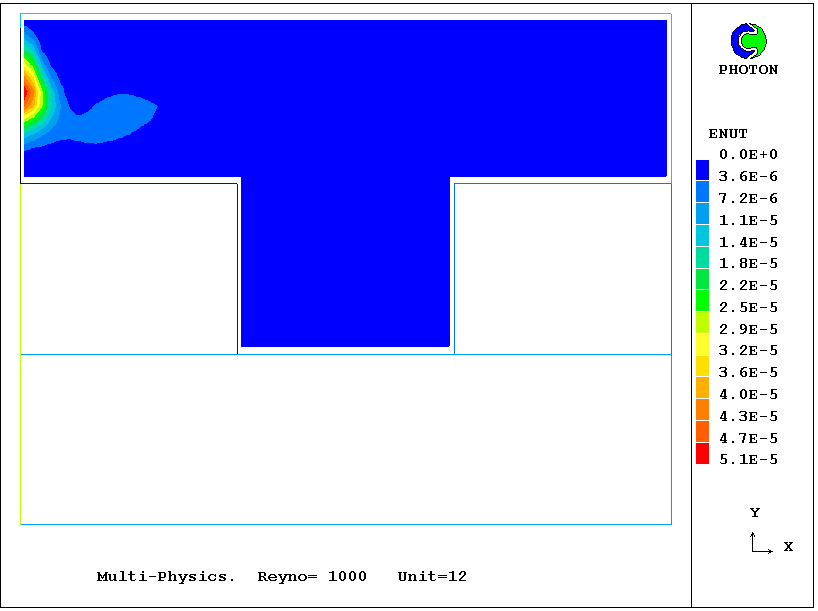
WDIS is calculated once for all, at the start of the computation.
From it, and from the developing velocity distribution, the
evolving distribution of ENUT, the effective (turbulent) viscosity
is derived.
The resulting contours of ENUT are shown in
Fig. 17.
Since the laminar viscosity is of the order of 1.e-5 m**2/s, it is
evident that turbulence raises the effective value, far from the
walls, by an order of magnitude.
next, back or
contents
(c) How the stresses were calculated
- As will be shown below, the equations governing the displacements are
very similar to those governing the velocities.
- The CFD code PHOENICS, like many others, can calculate velocities in
fluids; but this
ability is not
needed in the solid region; so such codes are usually idle there.
- However, PHOENICS can be "tricked" into calculating what it "thinks"
are velocities everywhere; whereas what it actually calculates in the
solid regions are displacements.
- The details of the "trickery" now follow.
next, back or
contents
3. The mathematics of the method
(a) Similarities between the equations for displacement and velocity
The similarities already referred to are here described for only one
cartesian direction, x; but they prevail for all three directions.
next, back or
contents
- The x-direction displacement, U, obeys the equation:
where:
- Te = local temperature measured above that of the un-stressed
solid in the zero-displacement condition, multiplied by
the thermal-expansion coefficient;
- D = [d/dx]* U + [d/dy]* V + (d/dz]* W
which is
called the "dilatation";
- Fx = external force per unit volume in x-direction;
- V and W = displacements in y and z directions;
- C1, C2 and C3 are functions of Young's modulus and
Poisson's ratio.
next, back or
contents
- When the viscosity is uniform and the Reynolds number is low, so that
convection effects are negligible,
the x-direction velocity, u, obeys the equation:
[del**2]* u - [d/dx]* [ p*c1 ] + fx*c2 = 0 ,
where
- p = pressure,
- fx = external force per unit volume in x-direction,
- c1 = c2 = the reciprocal of the viscosity.
next, back or
contents
Notes:
- The two equations are now set one below the other, so that they
can be easily compared:
- The equations can thus be seen to become identical if:
- p*c1 = D*C1 - Te*C3
which implies:
D = [p*c1 + Te*C3 ] / C1
- and
fx * c2 = Fx * C2
next, back or
contents
- The expressions for C1, C2 and C3 are:
- C1 = 1/(1 - 2*PR)
- C2 = 2*(1 + PR) / YM
where
- PR = Poisson's Ratio. and
- YM = Young's Modulus
and
- C3 = 2 *(1 + PR)/(1 - 2*PR)
next, back or
contents
- A solution procedure designed for computing velocities will
therefore in fact compute the displacements if:
- the convection terms are set to zero within the solid
region: and
-
the linear relation between:
- D ( ie [d/dx]* U + ...)
and
- p
is introduced by inclusion of a
pressure- and temperature-dependent "mass-source" term.
next, back or
contents
(b) Deduction of the associated stresses and strains
The strains (ie extensions ex, ey and ez) are
obtained from differentiation of the
computed displacements.
Thus:
ex = [d/dx]* U
ey = [d/dx]* V
ez = [d/dx]* W
next, back or
contents
Then the corresponding:
- normal stresses, sx, sy, sz, and
- shear stresses tauxy, tauyz, tauzx,
are obtained from the strains by way of equations such as:
sx = {YM / (1 - PR**2)} * {ex + PR*ey} and
tauxy = {YM / (1 - PR**2)} * {0.5 * (1 - PR)*gamxy}
where:
- gamxy = [d/dy]*U - [d/dx]*V
next, back or
contents
(c) The "SIMPLE" algorithm for the computation of displacements
PHOENICS employs (a variant of) the "SIMPLE" algorithm of Patankar &
Spalding (1972) for computing velocities from pressures, under a mass-conservation
constraint.
Its essential features are:
- All the velocity equations are solved first, with the
current values of p.
- The consequent errors in the mass-balance equations are computed.
- These errors are used as sources in equations for
corrections to p.
- The corresponding corrections are applied, and the process is
repeated.
next, back or
contents
All that it is necessary to do, in order to solve
for
displacements simultaneously, is, in solid regions, to treat the
dilatation B as the mass-source error and to ensure
that p obeys the above linear relation to it.
Therefore a CFD code based on SIMPLE can be made to solve the displacement equations
by:
- eliminating the convection terms (ie setting Re low); and
- making D linearly dependent on p and
temperatureT.
The "staggered grid" used as the default in PHOENICS proves to be extremely
convenient for solid-displacement analysis; for the velocities and
displacements are stored at exactly the right places in relation to
p.
next, back or
contents
4. Details of the auxiliary models
(a) IMMERSOL: summary
- The solved differential equation is:
div( effective_conductivity * T3 ) + source = 0
- effective conductivity =
0.75 * sigma * T3**3 / (abso + scat + 1/WGAP)
- source = abso * sigma * ( T1**4 - T3**4 )
- in solids, abso = large, so T3 --> T1
- surface resistances account for non-unity emissivities
next, back or
contents
Notes:
- The main novelty is the inclusion of WGAP, ie the distance
between the walls, in the formulae.
- This enables a conduction-type model to be used even with
non-participating media.
- Of course, an economical means of calculating WGAP is needed.
- This is provided by the LTLS equation (see below).
- IMMERSOL gives quantitatively correct predictions in geometrically
simple circumstances and plausible ones in complex ones.
- It is economical enough to be generalised for wavelength-dependent
radiation.
Click here
for more information.
next, back or
contents
(b) WGAP, WDIS and LTLS
- The solved differential equation is:
div (grad LTLS) = 1
The boundary conditions are:
LTLS = 0 , in all solids.
- The solution for plane channel flow is:
LTLS = WDIS * ( WGAP - WDIS ) / 2 , and
grad LTLS = WGAP / 2 - WDIS
- These relations are supposed to prevail also in two- and
three-dimensional circumstances.
- That is all!
next, back or
contents
Notes:
- The LTLS equation is very simple, and therefore easy to solve.
- Its solution yields values of LTLS and grad LTLS at
all points in the field.
- WDIS and WGAP are then deduced from them.
- Their values are quantitatively correct predictions in geometrically
simple circumstances and plausible in complex ones.
- The method is especially useful, indeed the only practicable one,
when the space in question contains many solids of arbitrary shapes.
Click here
for more information.
next, back or
contents
(c) LVEL: summary
next, back or
contents
Notes:
- The LVEL model is very simple, and therefore easy to implement.
- The predicted effective viscosities are quantitatively correct
in geometrically simple circumstances and plausible in complex
ones.
- The method is especially useful, indeed often the only practicable one,
when the space in question contains many solids of arbitrary shapes.
- LVEL handles the complete Reynolds-number range: laminar, transitional
and fully turbulent.
- LVEL can be easily extended so as to improve its accuracy in locations
far from walls.
Click here
for more information.
next, back or
contents
Click
here for an SFT example involving natural convection
next, back or
contents
5. Conclusions
The following conclusions appear to be justified:
- Simultaneous simulation of solid-stress, heat transfer and fluid flow
is indeed practicable and economical.
- As compared with the alternative, namely the use of distinct methods
for each phenomenon with iterative interaction between them, the
simultaneous-solution method is very attractive.
- It therefore seems possible that, when its attractiveness is fully
recognised, SFT (i.e. Solid-Fluid-Thermal) analysis may become as
popular as CFD.
next, back or
contents
- However, because older specialists have too-long believed the
two-distinct-method approach to be the only practicable one,
the future of the simultaneous-solution approach depends on its
adoption by younger ones.
- This is why it has been presented to the "School-Seminar for
Young Scientists".
next, back or
contents
- Such scientists, before committing themselves to this line of
research should ask:
- Is further research needed?
Answer:
Yes, in order to:
- establish whether the method truly predicts stresses
which agree with experimental findings;
- extend the method to problems in which the solid-fluid
interfaces intersect the computational-cell walls
obliquely;
- extend it to problems in which the displacements are not
small compared with the cell sizes;
- extend it also to non-linear and plastic-flow phenomena;
- discover and implement improvments to the numerical
method in respect of economy and accuracy.
next, back or
contents
- Is it speculative research, which may lead no where?
Answer:
No. There are no obstacles standing in the way of complete
success.
- Will contribution to such research guarantee a profitable
career in industry?
Answer:
Perhaps; but you will have at first to adjust yourself to a
world which does not believe, and perhaps does not want
to believe, that the simultaneous-solution method even exists.
next, back or
contents
- Wll it provide intellectual challenge and personal
satisfaction?
Answer:
Surely; for researchers in this field will have at first few
leaders to follow and few competitors to fear. They will be true
pioneers.
------------------------ END of LECTURE ------------------------
next, back or
contents
6. References
- The differential equations governing displacements, stresses and
strains in elastic solids of non-uniform temperature can be found
in numerous textbooks, for example:
- CT Yang
Applied Elasticity
McGrawHill, 1953
- BA Boley and JH Weiner
Theory of Thermal Stresses
John Wiley, 1960
- PP Benham, RJ Crawford and CG Armstrong:
Mechanics of Engineering Materials
Longmans, 2nd edition, 1996
It has not been common to choose the displacements as the
dependent variables in numerical-solution procedures. However, this
has been done by:
- JH Hattel and PN Hansen
A Control-Volume-based Finite-Difference Procedure for
solving the Equilibrium Equations in terms of
Displacements
Applied Mathematical Modelling, 1990
Their numerical procedure differ from that used here, which was that of
- SV Patankar and DB Spalding
"A Calculation Procedure for Heat, Mass and Momentum
Transfer in Three-Dimensional, Parabolic Flows"
Int J Heat Mass Transfer, vol 15, p 1787, 1972
- The first use of the present method for solving the solid-displacements
and fluid-velocity equations simultaneously appears to have been
made by CHAM, late in 1990.
Reports describing the early work include:
- KM Bukhari, HQ Qin and DB Spalding
Progress Report (to Rolls-Royce Ltd) on the Calculation of
Thermal Stresses in Bodies of Evolution
CHAM Ltd, November, 1990
- KM Bukhari, IS Hamill,HQ Qin and DB Spalding
Stress-Analysis Simulations in PHOENICS.
CHAM Ltd, May, 1991
From that time onwards, the solid-stress option was made available
as a (little-advertised) option in successive issues of
PHOENICS,
- Open-literature and conference publications have been few, but
include:
- DB Spalding
Simulation of Fluid Flow, Heat Transfer and Solid Deformation
Simultaneously
NAFEMS 4, Brighton 1993
- D Aganofer, Liao Gan-Li and DB Spalding
The LVEL Turbulence Model for Conjugate Heat Transfer at
Low Reynolds Numbers
EEP6, ASME International Mechanical Engineering Congress and
Exposition, Atlanta, 1996
- DB Spalding
Simultaneous Fluid-flow, Heat-transfer and Solid-stress
Computation in a Single Computer Code
Helsinki University 4th International Colloquium on Process
Simulation, Espoo, 1997
- DB Spalding
Fluid-Structure Interaction in the presence of Heat
Transfer and Chemical Reaction
ASME/JSME Joint Pressure Vessels and Piping Conference, San
Diego, 1998