last revised 08.08.22
FLAIR is a special-purpose program for Heating, Ventilation and Air Conditioning (HVAC) systems that are required to deliver thermal comfort, health and safety, air quality, and contamination control. FLAIR provides designers with a powerful and easy-to-use tool which can be used for the prediction of airflow patterns, temperature distributions, and smoke movement in buildings and other enclosed spaces. For example:
Figure 1.1 The computed temperature distribution in Hackney Town Hall
Figure 1.2 The temperature distribution in a computer room
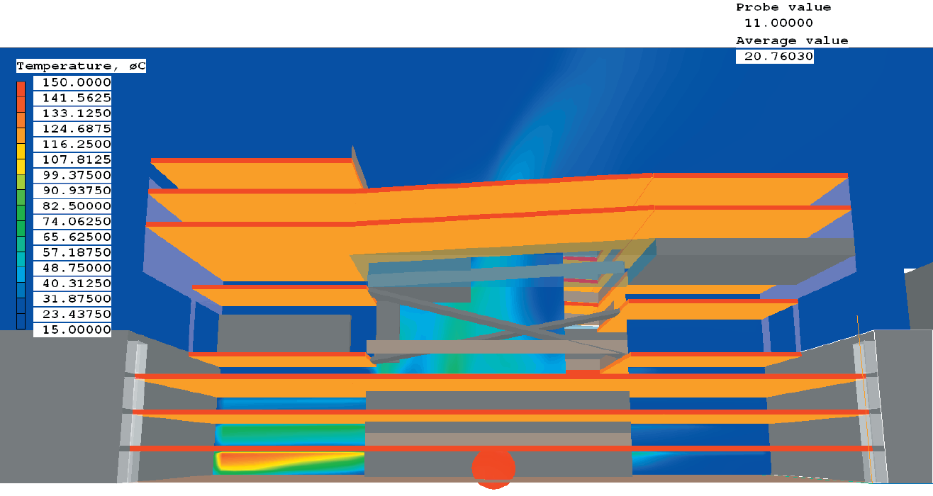
Figure 1.3 Temperature contours of the hot gases from a fire on a plane through the central space of a multi-storey car park (all temperatures above 100 degree C are shown in red)
Figure 1.4 Wind test over Melbourne cricket ground
As seen from above examples, FLAIR can be used during the design process to detect and avoid uncomfortable air speeds or temperatures. In addition, it can predict the effects of any gaseous pollutant, helping to achieve safe design of buildings, underground systems etc. It can also be used by various regulatory bodies and safety consultants.
FLAIR provides a state-of-art Virtual Reality User Interface for rapid model creation and visualisation of the results, including various thermal-comfort parameters. Little CFD knowledge is therefore required to operate FLAIR or to understand this guide. But the following warning should be heeded.
1.2 What FLAIR can assist its user to users to do
Many of the functions that are required to create a FLAIR model, to solve the problem, to examine the results and to activate on-line help, can be accessed through the single integrated FLAIR-VR interface.
1.3 What FLAIR users must do for themselves FLAIR can provide often-helpful default settings. But it cannot know what it has not been told; and its users must accept responsibility for the deciding what it should be told.
In the real world, floors are seldom smooth. In car parks they are usually of rough concrete, perhaps with raised ridges separating bays; in dwelling houses they may be carpeted; and grass or other vegetation is to be found out of doors. Only the user knows which is to be found, and where, in the scenario which it is hoped that FLAIR will realistically simulate.
FLAIR allows 'wall roughness' to be specified; but the user must estimate the magnitudes of the roughness lengths which are appropriate to the various surfaces.
In the majority of practical circumstances, solid objects and partitions are present which have thicknesses or surface irregularities which have too fine a geometrical scale to be realistically represented by the computational grid which covers the whole domain. It is the user who must decide whether FLAIR should ignore their existence; and, if not, which of its available devices should be activated to take approximate account of it.
For example, a metro-station platform may be crowded with people. The heat which they generate may be estimated and introduced to FLAIR as a volumetric heat source; and the space which they occupy by way of a volume porosity. But the effect of their presence on the flow of air is nor fully represented thereby; they exert resistances to the horizontal velocity components which require volumetric friction coefficients to be supplied also.
Similarly, car parks (by definition!) contain cars; and they certainly both provide a not-to-be-ignored resistance to the flow of air; and the eddies created between them augment the effective turbulent diffusion coefficients which FLAIR employs when calculating the distributions of temperature and pollutant concentration. That the FLAIR-VR interface happens to offer no specific means of representing these effects is no reason for ignoring them.
PHOENICS, the 'CFD engine' which underlies FLAIR, can represent the above phenomena by way of its In-Form (i.e. input-via-formulae) facility; but what formulae to employ? That the user must decide.
The decision is never easy to make; and for two reasons, namely:
What margin they decide to adopt is itself a matter of guesswork, must differ from scenario to scenario, and will vary from one aspect of a scenario to another. Rarely however will the reasonably cautious user feel confident in claiming limits closer than +/- 30%. Sometimes the range 10% to 1000% (for an essentially positive quantity) is more wisely accepted; and this is true not of FLAIR alone but of all predictive software based upon Computational Fluid Dynamics.
The just-mentioned choice of grid fineness has a big influence. Words to be found in tutorials such as "the grid will be generated automatically", may cause readers to suppose that PHOENICS will generate the optimum grid. But a moment's thought shows that to be impossible; for 'optimum' implies balance of advantages; and PHOENICS cannot know the relative importances which the user would assign to numerical precision, physical realism and economy of computer time.
PHOENICS will by default create a grid which does not completely over-look the presence of any of the distinct objects which the user has referred to; but often this produces a worst-of-both-worlds grid: too fine for economy and too coarse for accuracy.
The following image illustrates such a situation. The user wished to calculate the spread of smoke from a burning car in car park.
A better-instructed user would have:
Each run of FLAIR produces an alphanumeric RESULT file; and a few items likely to be of interest to HVAC users are supplied together with those which result from perhaps-unchanged PHOENICS-default settings. But the latter are many and the former few; so the user may miss what is intended for them.
PHOENICS possesses however a simply activated mechanism for printing the few items which the user selects into a single file (called INFOROUT); and this enables the user to see precisely what they want to see, and (for the moment) no more.
PHOENICS, and therefore FLAIR also, offers several graphical-display modules to its user. VR-Viewer, PHOTON and Win-PHOTON are among them; and it offers tutorial which teach users how utilise them. Less prominently described however is the means of not controlling them oneself (which requires skill, and is time-consuming); but instead causing their images to be created automatically by way of macros, i.e. commands written into a file which, when it receives it, the display package understands. All the PHOENICS packages can be operated in this manner.
The FLAIR user is therefore advised that, if they wish, they can do much more for themselves than FLAIR does automatically. One can find out about these from CHAM's User Support, from a more knowledgeable friend, or from the PHOENICS On-Line Information System, POLIS, accessible here (local) or here (online).
Every user makes mistakes at some time when inputting data, for example giving the gravitational acceleration a positive instead of a negative sign; or using kilojoules per second rather than watts for heat fluxes. The first may cause fluid to rise rather than sink; and the latter may cause generate physically improbable temperatures. But these implausible effects may escape the attention of the user who devotes it to one output item only; and PHOENICS cannot distinguish between intended and inadvertent inputs. Users are advised therefore first to take a 'bird's-eye view' of the simulated flow, and then to ask themselves: "Do I believe this?"
Qualitative features of the flow should correspond with expectations. Thus abrupt enlargements of the flow-cross-section should reveal recirculating-flow patterns downstream; and heavier fluids should fall below lighter ones. Most important is that the user should have expectations. If they do not they should ask a more experienced colleague. Users must not (to repeat the important point already made) rely on PHOENICS to proclaim: "Something's wrong."
PHOENICS does, by default, print information about the numerical accuracy of the calculation. Thus the nett mass source, i.e. the difference between the inflow and the outflow, is printed in the RESULT file. The user is advised to inspect it.
This chapter gives instructions for starting the FLAIR application. Following a simple example, you will use FLAIR to set up a problem, solve the problem and view the results. This is only a basic introduction to the features of FLAIR. Working through more tutorials described in Chapter 6 will provide a more complete demonstration of the program's features.
2.1 The Modes of FLAIR operation
The FLAIR pre-processor has several modes of operation. These are:
The 'VR-Environment' provides a graphical working environment in which users can run the FLAIR modules they wish, including Satellite, VR-Editor, Solver and VR-Viewer. It also provides mechanisms for:
The 'Satellite' mode is suitable for experienced users who do not wish to use the file-handling facilities provided by the VR-Environment, and are happy to run the individual modules from the system command line. The input Q1 file is read, and the EARDAT file for Earth is written after an (optional) interactive PIL command session.
For details about how to start FLAIR in the Satellite mode, the user is referred to PHOENICS document, Tr326. This document uses the FLAIR VR-Environment for this simple example.
2.2 Accessing the FLAIR on-line help
The Help button on the Help menu leads directly to this document and other documentation section of POLIS (PHOENICS On-line Information system) as shown below.
In FLAIR VR, information on the various hand-set control buttons can be displayed when the cursor is held stationary over any relevant control button. For example, when the cursor is held stationary over 'Menu' button, 'Domain attributes menu' will be displayed as shown below.
The following additional on-line help is available in the main menu of the FLAIR VR-Environment.
Click on the 'Help' button in the top menu for help on the main menu.
Click on the '?' in the top-right corner of any dialog box, then click on any input window or button to get information on the parameter which is set in it.
For example, if you want to obtain the information about Energy Equation,
'Temperature', click on the '?', ![]() in the top-right corner of any dialog box, then click on
'Temperature' button
in the top-right corner of any dialog box, then click on
'Temperature' button![]() , the following information will be displayed:
, the following information will be displayed:
Figure 2.1 shows the geometry of the example. The problem solved involves a room containing an air opening, a vent, a standing person, floor and walls held at a constant temperature. The room is 5m long, 3m wide, and 2.7m high. The opening measures 0.8 m x 1.0 m and allows cold air into the room to ventilate it. The vent is 0.8 m x 0.5 m, and extracts air at 0.2m3/s. The interaction of inertial forces, buoyancy forces, and turbulent mixing is important in affecting the penetration and trajectory of the supply air.
Figure 2.1 The simple example
We will take the following steps to set up the model:
The remaining sections provide step-by-step instructions on how to set up the model.
2.3.2 Setting up the model
Figure 2.2a The 'File' menu
Figure 2.2b 'Start New case' dialog
The FLAIR VR-Environment screen shown in figure 2.3 below should appear, which consists of two components: the Main window and the control panels (on the right).
Figure 2.3 The FLAIR-VR environment
FLAIR will create a default room with the dimensions 10m x10m x3 m, and display the room in the graphics window.
You can rotate, translate, or zoom in and out from the room by clicking the 'Mouse' button on the movement control panel and then using left or right mouse buttons.
Figure 2.4 Resize the default room to 3mx5mx2.7m on the control panel
The resized room shown in figure 2.5 will appear on the screen.
Figure 2.5 The resized room
2,3.4 Adding objects to the room
a. Make all the domain edges friction boundaries.
Figure 2.6 The Main Menu
Figure 2.7 The Domain Edge Dialog
Figure 2.8 The Heated Wall
b. add the next object, which will act as a person in the room.
Figure 2.9 The Object management dialog Box.
Figure 2.10 The Object specification dialog box
Figure 2.11 The PERSON's attributes panel
Set:
Body width: 0.6 m
Body depth: 0.3 m
Body height: 1.76 m
Figure 2.12 The standing man's attributes
Click on 'OK' to return to 'Object Specification' dialog box.
X: 1.5 m
Y: 2.0 m
Z: 0.0 m
Click on 'OK' to close the dialog box.
c. Next add a vent.
X:0.8 m
Y:0.0 m
Z:0.5 m
X: tick 'At end'
Y: 0.0 m
Z: 0.0 m
d. Next add an Opening:
X:0.8 m
Y:0.0 m
Z:1.0 m
X: 1.19 m
Y: tick 'At end'
Z: 1.5 m

Figure 2.13 The screen picture after all the object were created
To activate the physical models
a. The Main Menu panel
 .
The top page of the main menu, as shown in figure 2.14, will
appear on the screen. The menu date may differ from that shown.
.
The top page of the main menu, as shown in figure 2.14, will
appear on the screen. The menu date may differ from that shown.
Figure 2.14 The Main Menu top page.
While this panel is on the screen, you may set the title for this simulation, click on the 'Title' dialogue box. Then type in a suitable title, for example 'My first flow simulation'.
FLAIR always solves pressure and velocities. The temperature is also solved as the default setting.
Figure 2.15 The 'Models' page of the Main Menu.
b. To activate LVEL turbulence model
Figure 2.16 Select LVEL on the "Turbulence Models" page of the Main Menu.
To set the grid numbers and solver parameters
- 58 cells in the X-direction
- 46 cells in the Y-direction
- 54 cells in the Z-direction
Figure 2.17 Geometry menu page
This mesh is too fine for the example, as we wish to minimise the run-time, but may need to be refined for a more accurate solution. We can reduce the number of cells by changing the automeshing rules.
Figure 2.17a Automesh settings
The full function of the Grid Mesh Settings dialog is explained in TR326.
Set the number of sweeps in this window to 500 as shown in figure 2.18.
Figure 2.18 Set the " Total number of iterations' to 300
Figure 2.19 Monitoring position
It can also be set by clicking on 'Output' on the main menu. For this case, the monitor-cell location, (18,16,10) will be displayed.
FLAIR uses the PHOENICS solver called 'Earth'.
To run Earth, click on 'Run', and then 'Solver', followed by clicking 'OK' to confirm running Earth. These actions should result in the PHOENICS Earth screen appearing.
As the Earth solver starts and the flow calculations commence, two graphs should appear on the screen. The left-hand graph shows the variation of pressure, velocity and temperature at the monitoring point that was set during the model definition. The right-hand graph shows the variation of errors as the solution progresses.
As a converged solution is approached, the values of the variables in the left-hand graph should become constant. With each successive sweep number, the values of the errors shown in the right-hand window should decrease steadily.
Figure 2.19 shows the EARTH monitoring screen at the end of the calculation.
Figure 2.20 The EARTH run screen at the end of calculation
Runs can be stopped at any point by following the procedure outlined below.
Please note: if the solver is stopped before the values of the variables in the left-hand graph of the convergence monitor approach a constant value, the solution may not be fully converged, and the resulting flow-field parameters may not be reliable.
2.3.4 Viewing the Results with VR-Viewer
The results of the flow-simulation can be viewed with the FLAIR VR post-processor called VR-Viewer.
In the VR-Viewer, the results of a flow simulation are displayed graphically. The post-processing capabilities of the VR-Viewer that will be used in this example are:
To access the VR Viewer, simply click on the 'Run' button, then on 'Post processor', then 'GUI Post processor (VR Viewer)' in the FLAIR-VR environment.
When the 'File names' dialog appears, click 'OK' to accept the 'latest dumped' result files. The screen shown in figure 2.20 should appear.
Figure 2.20 The VR-Viewer screen picture as it appears for this case.
Viewing the Results with VR-Viewer
The detailed description of the VR-Viewer screen and hand set control buttons is provided in PHOENICS documentation TR326. This section simply gives instructions on how to view the results.
To view the results of the simple simulation just completed:
Figure 2.21 Stream Options dialog box
Typical displays of a vector, contour and a streamlines plot are shown below in figures 2.22 (a - c) respectively.
Figure 2.22a Vector plot.
Figure 2.22b Contour plot.
Figure 2.22c Streamlines.
2.3.5 Printing from VR.
Screen images such as figures 2.22(a - c) can be sent directly to a printer by clicking on 'File', then on 'Print' from the main environment screen. A dialog similar to that shown in figure 2.23a opens.
Figure 2.23a Print Dialog Box
Alternatively, the screen image can be saved to a file by clicking on 'File', then on 'Save window as' from the main environment screen.
When 'Save window as' has been pressed, the dialog box shown in figure 2.23b opens.
Figure 2.23b 'Save Window as' Dialog Box
The 'Save as file' dialog offers a choice between GIF, PNG, BMP and JPG file formats, and allows the image to be saved with a higher (or lower) resolution than the screen image. (An image can be saved in PCX format by adding the '.pcx' extension to the file name.)
The graphics files are dumped in the selected folder (directory), with the given name. In all cases, the background colour of the saved image is that selected from 'Options', 'Background colour' from the VR-Editor main environment screen.
The above example has been designed to show how to use FLAIR to solve a very simple problem. More examples are provided in chapter 6, Tutorials, where how to use the different modeling objects, physical models and post-processing capabilities that are available in FLAIR are described in more detail.
FLAIR provides seven active HVAC-specific object types, Diffuser, Fire, Jetfan, Spray-head, Rain, Person, People, one external windflow object type TERRAIN and two post-processing objects ROOM / AIRVOL and Raingauge as described below.
The Diffuser is a single object representing a complex source of mass, momentum and energy. It is used to represent various types of diffusers found in rooms and buildings. The detailed implementation is based on the 'Momentum method' described in ASHRAE Report RP-100915.
The diffuser object can be accessed through the Object management dialog box. To load a diffuser object, click on the 'Obj' button on the main control panel to bring up the Object management dialog box. Then click on 'Object' , 'New' and 'New object' pull-down menu to bring up the Object specification dialog box. Select Diffuser from object 'Type' as shown in figure 3.1.
Figure 3.1 Selecting Diffuser from the object 'Type'
The default diffuser is the 4-way diffuser. Figure 3.2 shows the default diffuser attributes.
Figure 3.2 The default diffuser and its attributes
The following specifications can be defined through the attributes panel:
Diffuser type - there are 5 different types as shown in figure 3.3. Each type has its own shape.
Figure 3.3 The select diffuser type panel
The diffuser types have the following characteristics:
Figure 3.4 Round diffuser
Figure 3.5 Vortex diffuser, 45deg swirl angle.
Figure 3.6 4-way rectangular diffuser
Figure 3.7 4-way directional diffuser, all faces active
Figure 3.8 Grille diffuser, 45 deg symmetrical deflection
Figure 3.9 Displacement diffuser, 4 sides and top face active
Diffuser Attributes
All diffuser types can be rotated freely about any axis or combination of axes. Note however that if Grille, Round, Vortex or 4-way rectangular diffusers are rotated out of the plane of the grid, they must lie on the face of a BLOCKAGE object otherwise they will produce no flow.
Diffuser position - for all diffusers other than displacement, these set the coordinates of the centre of the mounting face of the diffuser. For displacement diffusers, it sets the low x,y,z corner.
Diffuser diameter - for round and vortex diffusers, this sets the diameter of the diffuser.
Diffuser size - for rectangular diffusers, sets the length of the faces.
Plane - This allows the user to place the diffuser in the X, Y or Z planes.
Side - When the diffuser is mounted internally in the solution domain, the diffuser itself can be on the decreasing-coordinate (low) or the increasing-coordinate (high ) side of the mounting face. The position boxes set the location of the mounting face - this controls whether the diffuser is above or below, to the left or right.
X/Y/Z Faces - For 4-way directional and displacement diffusers, these control which faces of the diffuser are active. The supply volume is divided uniformly amongst the active faces.
The face directions and deflection angles referred to below are always in the coordinate system of the diffuser itself, not taking into account any rotations. For example, consider a 4-way directional diffuser in the X-Y plane which has been rotated +90deg about Z. The high X face of the diffuser will now point along Y.
Supply pressure - This sets the pressure of the supply air, relative to the Reference Pressure set on the Properties panel of the Main menu (usually 1.01325E5 Pa). It is used together with the supply temperature to calculate the density of the supplied air. By default it is set to the ambient pressure, which is also set on the Properties panel. Any other value can be entered by switching to 'User'.
Supply temperature - This sets the temperature of the supply air in degree C. By default, it is set to the ambient temperature, which is set on the Properties panel of the Main menu. Any other value can be entered by switching to 'User'.
Supply volume - This sets the volumetric flow rate for the supply air in L/s or m3/s.
Set throw or effective area - The diffuser can be defined either in terms of the Effective area or Throw and terminal velocity. These factors are usually obtained from manufacturer's data sheets.
The Effective area can be deduced by dividing the supply volume flow rate by the discharge velocity. It is always less than the nominal plan area.
If the Throw and terminal Velocity are set, the discharge velocity and hence Effective area are deduced using a jet formula and the jet decay constant.
The depth of the diffuser (except grille and displacement) is deduced by dividing the Effective area by the active perimeter.
The diffuser object introduces mass and three components of momentum as sources. The mass source and normal-to-surface velocity is taken from the user-set volume flow rate divided by the actual area of the object. The parallel-to-surface velocity components are taken from the volume flow rate divided by the user-set effective area.
The angle of the resulting flow away from the normal can be shown to be:
ang = atan(Aactual/Aeffective)
so to set an angle to normal, the 'Effective area' should be set to the actual area divided by the tan of the angle.
Note that the actual area to be used is just the diameter squared, leaving out the π/4 part, as internally the round diffuser is represented as being square.
Swirl angle (for Vortex type only) - This sets the amount of swirl induced by the diffuser. A value of zero gives no swirl (equivalent to a round diffuser); the flow is purely radial. A value of 90 means the flow is purely tangential. Positive angles produce anti-clockwise swirl when looking down on the diffuser. This is usually the angle the diffuser blades are set to.
Angles from Z axis (for Grille/Nozzle type only) -
Figure 3.10 The Grille diffuser and its attributes
This specifies the deflection from the normal to the plane of the diffuser in each of the other two directions. If the plane is The default value of 0.0 means no deflection- the flow comes out normal to the diffuser surface. Positive values mean deflection in the + axis direction; negative values mean deflection in the - axis direction. The deflection is limited to +/- 89 degrees.
When the Symmetric Yes/No switch is set to Yes, the flow is divided symmetrically in the positive and negative axis directions. It is as if the grille were made up of two grilles with opposite deflection angles. When set to No, both halves use the same deflection angle. As the grille is divided horizontally and vertically, there are actually four sources for each grille.
Effective area ratio (for displacement type only) - For a displacement diffuser, this is the ratio between the true flow area and the modeled area. It is the same for all active faces.
The fire object is used to create an area or volumetric heat source, representing a fire. There are several options for setting the heat, mass and smoke sources at the fire. It is assumed that the mass released by the fire is the products of combustion, and that the SMOK variable represents the local mass fraction of combustion product.
Some combinations require the Heat of Combustion Hfu and the stoichiometric ratio, Rox to be set. If the product mass-fraction SMOK is solved, these values are set in Main menu - Solve smoke mass fraction - settings. If SMOK is not solved, these settings can be made on the Fire object dialog.
The details of how the heat source is specified depend on the fire model selected in the Main menu - Solve smoke mass fraction - settings dialog.
The fire can be loaded through the Object management in the same way as described in section 3.1 above for the diffuser.
The available fire models are:
The default fire object and its attributes are shown in figure 3.11 below.
Figure 3.11 The fire and its default attributes
The dialog will change as different options are selected, showing input boxes for the various parameters.
Heat Source
The heat source set here is the total heat source Qt =Qconvective + Qradiative. If the radiation model is not active, the heat source reported in the solution (as 'Source of TEM1') is reduced by the Radiative fraction Rf to be just the convective part. The Radiative factor is set on the 'Smoke settings' panel of the Main Menu, and is defaulted to 0.3333. The total heat release rate is still used to derive the smoke mass source
The options for the Heat source are:
Figure 3.12 Fire heat sources
Qt = mass*Heat of Combustion / (1+Rox)
If the Heat of Combustion is not constant, use 'From table file' for both the heat and mass sources.
Qt = a + b*(T+TEMP0)
where TEMP0 is the reference temperature.
If T is below Tmin or above Tmax, these values are used in the formula.
Qt = min(Qmax, a*(t-t0)b)
where Qmax is the maximum permitted heat release rate, t0 is the time at the start of the fire, and a and b are constants.
It has been found that the heat release rate grows approximately as the square of the time i.e. the b constant above is 2.0. Characteristic growth times and constants for various classes of fire are given in Table 10.1 of the CIBSE Guide E, Fire Engineering (Ref 4).
| Fire class | Characteristic growth time (s) |
Constant a (W/s2) |
| Ultra-fast | 75 | 187.6 |
| Fast | 150 | 46.9 |
| Medium | 300 | 11.7 |
| Slow | 600 | 2.9 |
Qt = Q(n-1) +(t-t(n-1)) / (t(n)-t(n-1))*(Q(n)-Q(n-1))
Time,Qt
0,   0
60,  350000
120, 700000
180, 1050000
240, 1400000
300, 1400000
360, 1400000
420, 1400000
480, 1400000
540, 1400000
600, 2055000
The Earth solver will perform a linear interpolation in the table to find the heat source for any particular time. The time in the table is the time since ignition. This option allows for any number of points in the table, and should be used in preference to 'Piece-wise Linear in time' if there are more than 10 points.
In a transient case, a file called 'heat_sources.csv' will be created. It will contain the convective heat source for each fire object for each time step. An example is given here:
Time ,     FIXMAS ,   POOL ,     PWLM ,     FIXT ,     FIXQ ,     LINTEM ,
3.000E+01, 1.100E+05, 7.705E+05, 1.719E+03, 0.000E+00, 1.320E+06, 1.005E+05,
9.000E+01, 1.100E+05, 1.346E+06, 5.156E+03, 2.747E+05, 1.320E+06, 1.005E+05,
1.500E+02, 1.100E+05, 2.011E+06, 8.594E+03, 2.747E+05, 1.320E+06, 1.005E+05,
2.100E+02, 1.100E+05, 2.753E+06, 1.203E+04, 2.747E+05, 1.320E+06, 1.005E+05,
2.700E+02, 1.100E+05, 3.561E+06, 1.547E+04, 5.493E+05, 1.320E+06, 1.005E+05,
The first column is the solver time, at the mid-point of each time step. The subsequent columns are the heat release rates in Watts for the FIRE objects named in the first row.
Mass Source
The options for the Mass source are:
Figure 3.13 Fire mass sources
The mass released is taken to be the products of combustion:
1kg Fuel + Rox kg Oxygen = (1+Rox) kg Product
Mass = Qt * (1+Rox) / Heat of Combustion
If the Heat of Combustion is not constant, use 'From table file' for both the heat and mass sources.
Area = a + b * tc
Mass = Area *( 1-exp(-B*Area.5))
Mass=M(n-1) +(t-t(n-1)) / (t(n)-t(n-1))*(M(n)-M(n-1))
Time, Mass
0,    0
60,   0.0073
120,  0.0219
180,  0.0365
240,  0.051
300,  0.0583
360,  0.0583
420,  0.0583
480,  0.0583
540,  0.0583
600,  0.072
The Earth solver will perform a linear interpolation in the table to find the mass source for any particular time. The time in the table is the time since ignition. This option allows for any number of points in the table, and should be used in preference to 'Piece-wise Linear in time' if there are more than 10 points.
In a transient case, a file called 'smoke_sources.csv' will be created. It will contain the product mass (smoke) source for each fire object for each time step. An example is given here:
FIXMAS ,POOL ,PWLM , FIXT , FIXQ , LINTEM ,
3.000E+01, 2.000E-02, 1.401E-01, 3.125E-04, 8.182E-05, 2.400E-01, 1.828E-02
9.000E+01, 2.000E-02, 2.446E-01, 9.375E-04, 8.182E-05, 2.400E-01, 1.828E-02
1.500E+02, 2.000E-02, 3.656E-01, 1.562E-03, 8.182E-05, 2.400E-01, 1.828E-02
2.100E+02, 2.000E-02, 5.005E-01, 2.187E-03, 8.182E-05, 2.400E-01, 1.828E-02
2.700E+02, 2.000E-02, 6.474E-01, 2.812E-03, 8.182E-05, 2.400E-01, 1.828E-02
The first column is the solver time, at the mid-point of each time step. The subsequent columns are the mass release rates in kg/s for the FIRE objects named in the first row.
Scalar Source
The options for the Scalar source are:
Figure 3.14 Fire smoke sources
The SMOK scalar is taken to be product of combustion - the inlet value is therefore always 1.0. The parameters determining how the smoke concentration affect visibility are all set in Main menu - Solve smoke mass fraction - settings.
mass = Qt (1+ Rox)/ Heat of Combustion
This is then used to set the scalar source.
Note that some of the source types are only available for transient simulations. Not all source types are mutually compatible - for example if the mass source is 'heat related', the heat source cannot be 'mass related'. Such incompatible combinations will be flagged up as errors when trying to set them.
InForm - InForm sources are set through the InForm Commands button. This leads to a dialog from which a selection of InForm commands can be attached to this object. It is described here.
Dutch NEN 6098 Standard
The default fire object and its attributes for the Dutch NEN 6098 Standard are shown below.
Heat Source
The heat source set here is the total heat source Qt =Qconvective + Qradiative. If the radiation model is not active, the heat source reported in the solution (as 'Source of TEM1') is reduced by the Radiative fraction Rf to be just the convective part. The Radiative factor is set on the 'Smoke settings' panel of the Main Menu, and is defaulted to 0.3. The total heat release rate is still used to derive the smoke mass source
The options for the Heat Source are:
Time,Qt
0,   0.
60,  350000
120, 700000
180, 1050000
240, 1400000
300, 1400000
360, 1400000
420, 1400000
480, 1400000
540, 1400000
600, 2055000
The Earth solver will perform a linear interpolation in the table to find the heat source for any particular time. The time in the table is the time since ignition.
In a transient case, a file called 'heat_sources.csv' will be created. It will contain the convective heat source for each fire object for each time step.
Mass Source
The mass source is set to Heat Related - the mass source is deduced from the total heat source by dividing by a heat of combustion
Mass = Qt * (1+Rox) / Heat of Combustion
In a transient case, a file called 'smoke_sources.csv' will be created. It will contain the product mass (smoke) source for each fire object for each time step.
Scalar Source
The SMOK scalar is taken to be product of combustion - the inlet value is therefore always 1.0. The parameters determining how the smoke concentration affect visibility are all set in Main menu - Solve smoke mass fraction - settings.
The Scalar Source is set to Mass-related - the rate of scalar release is linked to the mass release rate.
InForm - InForm sources are set through the InForm Commands button. This leads to a dialog from which a selection of InForm commands can be attached to this object. It is described here.
Belgian NBN S 21-208-2/A1 Standard
The default fire object and its attributes for the Belgian NBN S 21-208-2/A1 are shown below.
Heat Source
The heat source set here is the total heat source Qt =Qconvective + Qradiative. If the radiation model is not active, the heat source reported in the solution (as 'Source of TEM1') is reduced by the Radiative fraction Rf to be just the convective part. The Radiative factor is set on the 'Smoke settings' panel of the Main Menu, and is defaulted to 0.34. The total heat release rate is still used to derive the smoke mass source
The options for the Heat Source are:
Time,Qt
0,   0.
60,  350000
120, 700000
180, 1050000
240, 1400000
300, 1400000
360, 1400000
420, 1400000
480, 1400000
540, 1400000
600, 2055000
The Earth solver will perform a linear interpolation in the table to find the heat source for any particular time. The time in the table is the time since ignition.
Mass Source
The mass source is set to Heat Related - the mass source is deduced from the total heat source by dividing by a heat of combustion
Mass = Qt / Heat of Combustion
In a transient case, a file called 'smoke_sources.csv' will be created. It will contain the product mass (smoke) source for each fire object for each time step.
Scalar Source
The SMOK scalar is taken to be burnt fuel - the inlet value is therefore always 1.0. The parameters determining how the smoke concentration affect visibility are all set in Main menu - Solve smoke mass fraction - settings.
The Scalar Source is set to Mass-related - the rate of scalar release is linked to the mass release rate.
InForm - InForm sources are set through the InForm Commands button. This leads to a dialog from which a selection of InForm commands can be attached to this object. It is described here.
The jetfan object is used to create a volume of fixed velocity, representing the effects of a jetfan. The velocity components in the domain X-, Y- and Z-axes are calculated internally to give the set total velocity and direction.
The jetfan can be loaded through the Object management in the same way as described in section 3.1 above for the diffuser.
The default jetfan object and its attributes are shown in figure 3.15 below.
Figure 3.15 The jetfan and its default attributes
Fan type - The fan can be rectangular or circular in cross-section. Unless the grid is very fine, the difference will be mainly visual.
Xpos, Ypos, Zpos - Sets the location of the centre of the jetfan object. Any rotations set will be about this point.
Length - Sets the length of the jetfan in the X co-ordinate direction of the jetfan.
Width - Sets the width of a rectangular jetfan in the Y co-ordinate direction of the jetfan.
Depth - Sets the depth of a rectangular jetfan in the Z co-ordinate direction of the jetfan.
Diameter - Sets the diameter of a circular jetfan.
Velocity - Sets the delivery velocity of the jetfan in the X co-ordinate direction of the jetfan. The jetfan always blows along its own X-axis. The jetfan can be rotated about its centre to point in any desired direction.
Set turbulence intensity - when Yes, sets the turbulence intensity for the jetfan. Typical values may be in the range 20 - 25%. The turbulence quantities are set from:
KEjet = (Intensity/100 * Velocity)2 ; EPjet = 0.1643*KEjet3/2/(0.1*diameter)
For a rectangular jetfan, the diameter is taken as 0.5*(Height+Width).
When No, the jetfan has no direct impact on the turbulence field other than by creating additional velocity gradients.
The default setting is No. When switched to Yes, a value of 22% is set.
Heat load - Sets the heat gain (or loss) through the jetfan. The default setting of 0.0 ensures there is no heat gain or loss. Positive values represent a heat gain, as through a heater, negative values represent a loss, as through a cooler.
Angle to X axis - Sets the inclination of the jetfan X co-ordinate to the domain X-axis. The resulting flow direction is as shown in the table below:
| Angle | Jet direction |
| 0 | +X |
| 90 | +Y |
| 180 | -X |
| 270 | -Y |
Angle to Z axis - Sets the inclination of the jetfan X co-ordinate to the domain Z-axis. The default angle of 90 directs the jet parallel to the floor. Angles > 90 incline the jet towards the floor, angles < 90 incline the jet towards the ceiling.
The spray-head is the sprinkler designed for fire extinction. It works with the GENTRA 22 module (see Encyclopaedia in POLIS). The spray-head can be loaded through the Object management in the same way as described in section 3.1 above for the diffuser.
The default spray-head object and its attributes are shown in figure 3.16 below.
Figure 3.16 The default spray-head object
The following specifications can be defined in the attributes dialog box:
Spray axis direction - This sets the axis of the spray to be along the positive X, Y or Z axis. The spray-head disk is normal to the selected axis.
Spray position - This sets the location of the centre of the spray-head disk. The disk is always normal to the spray axis.
Spray radius - This sets the radius of the spray-head disk. The droplet injection ports are uniformly distributed along the circumference of the disk.
Number of ports - This sets the number of the injection ports around the circumference of the spray disk.
Total volume flow rate - This sets the total volumetric flow rate of the water to be injected from the spray. The total amount is divided equally among the injection ports. The units are always litres/second.
Total injection velocity - This sets the velocity with which the droplets are deemed to be injected.
Spray angle (from spray axis) - This sets the angle between the spray and the spray axis. When set to 0.0, the droplets will be injected in the direction of the positive spray axis. Usually this will mean vertically upwards. When set to 90, the droplets will be injected normal to the axis. Usually this will mean horizontally. When sets to 180, the droplets will be injected in the direction of the negative spray axis. Usually this will mean vertically downwards.
Injection temperature - This sets the temperature of the injected droplets. The units are always degree C.
Volume median diameter - 50% of the water, by volume, is contained in droplets of this or greater diameter. Other 50% is contained in smaller droplets.
Number of size ranges - This sets number of droplet size to be considered. When sets to 1, the droplets will take volume median diameter. When sets to greater than 1, the sizes used will lie between the set minimum and maximum values, and will be distributed according to the Rosin-Ramler droplet distribution function.
Calculate link temperature (appears for transient run only) - This determines whether the link temperature for the spray will be calculated or not. If 'Calculate link temperature' is set to 'Yes', then two more entries, Activation temperature and Response time Index, will appear. The Track start- and end-times will be reset to 'Auto-on', and a new data entry box will appear for setting the duration of the spray after initiation.
Activation temperature is the temperature at which the track is to start.Response Time Index (RTI) is a measure of the detector sensitivity.
The link temperature is calculated from17:
dTl/dt = √(|Vel|) (Tg-Tl/) / RTIwhere Tl is the link temperature, Vel is the gas velocity and Tg is the gas temperature.
The calculated link temperatures are written to the file 'tlink1'csv' at the end of each time step. If there are more than 20 sprays, each group of 20 will be written to a separate 'tlinkn.csv' file where n is 1,2,3 etc.
A tutorial is provided in section 6.9 which shows how to use the Spray-head object for the simulation of fire extinction.
If GENTRA is not active at the time the first spray-head object is created, it will be automatically turned on, with all settings made for the spray model. Only the spray start- and end-times need be set for a transient case, should the spray not be active all the time.
If GENTRA is already turned on, it will be assumed that all settings are correct, and no default settings will be made.
The settings made for GENTRA are:
The rain object in effect represents a rain-producing area of sky. It works with the GENTRA 22 module (see Encyclopaedia in POLIS). The rain object can be loaded through the Object management in the same way as described in section 3.1 above for the diffuser.
The default rain object and its attributes are shown in figure 3.16a below.
Figure 3.16a The default rain object
Each ball represents a GENTRA droplet injection port. Each port can emit up to five droplets of different diameters.
The attributes have the following meanings:
Number of ports (X) - sets the number of ports in the X direction.
Number of ports (Y) - sets the number of ports in the Y direction.
The rain object is assumed to be zero thickness in Z, and to extend in the X and Y directions. However, it can be freely rotated about the X, Y and Z axes from the object Place page. The shape is restricted to a rectangle.
Total rain flowrate - sets the rain flowrate from this object in mm/hr. The total flowrate is evenly distributed amongst all the droplet sizes from this object. Typical flowrates might be:
Number of droplet sizes - sets the number of droplet sizes emitted by each port. Up to five sizes can be specified. To specify more than one size, enter the required number of sizes and click 'Apply'. New input boxes will appear for the set number of sizes.
Diameters - sets the diameter(s) of each droplet in mm. The diameter of the first droplet size is initially deduced from the total rain flowrate using the expression:
Diam= 1.105*(Flow rate)0.232 (Ref 23)
Horizontal components of rain velocity - sets a common horizontal initial velocity for all droplets. This will commonly be the horizontal components of the wind velocity at the injection height. The vertical velocity component is deduced from the droplet size as the terminal fall velocity using the expression:
W = -9.4*(1 - e-(Diam/1.77)1.147) (Ref 24)
Link airflow to tracks - the airflow will always affect the paths of the rain droplets. When this box is not ticked, it is assumed that the droplets do not influence the air flow. If it is ticked, then the full two-way interaction is implemented.
If GENTRA is not active at the time the first rain object is created, it will be automatically turned on, with all settings made for the rain model. Only the rain start- and end-times need be set for a transient case, should the rain not be active all the time.
If GENTRA is already turned on, it will be assumed that all settings are correct, and no default settings will be made.
The settings made for GENTRA are:
The Person object represents the heat load effect of a single human being. It does not apply a resistance to motion.
Figure 3.17 The default Person object
The 'Posture' button allows a choice of 'Standing' (as in the image above), 'Sitting' or 'User'. If 'User' is selected, the Size and Position dialogs on the Object Specification dialog can be used to size and rotate the image. The 'Facing' button toggles through +X,-X,+Y and -Y to determine which direction the person faces.
The heat source can be Total heat in W, of fixed temperature in Centigrade.
The People object is used to represent the heat load of a large number of people, for example the audience in a theatre. It does not apply a resistance to motion.
Figure 3.18 The default People object
The TERRAIN object is provided for external wind-flow cases where the surrounding terrain is not flat. The default shape is rectangular (box.dat), but any geometry including CAD imports can be used. There is no limit on the number of TERRAIN objects in a model.
It is designed to be used in conjunction with the WIND object, which supplies the incoming wind boundary layer, fixed pressure outflows and potentially ground surface temperatures. The WIND profile always starts from the upper surface of any TERRAIN object. TERRAIN objects at the domain boundary that do not align with the domain boundary should extend beyond the domain so as not to act as an unphysical vertical 'cliff'. This can be done once the 'Constrained by the domain' toggle is turned off.
The TERRAIN object is almost identical to a BLOCKAGE object with the following differences:
The ROOM object is used to define a volume of space, which may physically be a room in a building, or just any volume of space. For this reason, AIRVOL can be used as a synonym for ROOM.
The Earth solver will calculate the volume of the object, excluding any solid obstructions, and sum up the volumetric inflow rate across the boundary of the object, including any internal air supply. It will then print into the RESULT file the number of Air Changes per Hour for the volume defined by the object. This is calculated from 3600.0*(sum of volumetric inflows)/(room volume). The ROOM object has no effect on the solution.
By default, the ROOM / AIRVOL object is represented as a transparent cuboid, but it can be given any required shape, for example the CAD representation of the inside of a room.
Figure 3.18a The default ROOM / AIRVOL object dialog
In addition, the ROOM / AIRVOL object can:
The Air Exchange Effectiveness is then defined as the average AGE2 at outflow from the ROOM divided by the average AGE2 within the ROOM / AIRVOL.
If 'Store Air Exchange Efficiency' is ticked, then a 3D variable called AEE is created, and is filled with the Air Exchange Efficiency for the ROOM / AIRVOL. All cells within a ROOM / AIRVOL will have the same value. The Viewer will only plot AEE values within ROOM / AIRVOL objects.
A typical output is shown here:
 For object ROOM1
 ---------------------
 Overall residence time calculated as
 free volume/volum.flow-rate (in seconds)
 RES.TIME=15.756434
 Ventilation rate in air changes per hour
 ACH =228.478088
 The total free volume in the room is (m^3)
 VOLUME =1639.037354
 The total volumetric flow rate is (m^3/s, m^3/hr)
 VFLRT s =104.023369 ;VFLRT h=3.744841E+05
 The total internal volumetric source is (m^3/s, m^3/hr)
 VFLRT s =20.00001 ;VFLRT h=7.200003E+04
 The volume-weighted average temperature
 Ave Temp=21.348534
 The minimum and maximum temperatures
 Min Temp=20.012905 ;Max temp=26.051905
 The Air Exchange Effectiveness
  i.e. (ave outflow local age)/(ave local age in room)
 AEE=0.42062

 The local Air Change Effectiveness
  i.e. RES.TIME/(average local age for room)
 Local Mean Age of Air for room
 MAA local=6.559762
 ACE local=2.401983

 The global Air Change Effectiveness
  i.e. RES.TIME/(average domain age for room)
 Global Mean Age of Air for room
 MAA global=7.085855
 ACE global=2.223646

 The area-averaged absolute velocity at 1.6m
 VAB_AVE=3.173288
 The total free area of the room is (m^2)
 AREA =327.005737
The same information can be obtained in the Viewer by right-clicking on a ROOM object and selecting 'Show nett sources' from the context menu that appears. The data is then also written to a file called 'ACH results for object name at sweep n.txt', where name is the name of the object and n is the sweep number.
3.10 Raingauge (Track_counter)
The raingauge object is used to define a surface. The default shape is a cuboid, but any desired shape can be used. It counts the number of Rain tracks or Spray-head droplets passing through (only the entry point is noted), and reports the total mass passing through (entering) the object.
The Raingauge object only exists in Flair. In Core PHOENICS there is an equivalent Track_counter object which performs the same functions. It can also be created in the Viewer, unlike the Raingauge.
In the Editor, the Attributes dialog is not accessible. In the Viewer, the Raingauge attributes dialog appears as shown below:
Figure 3.18a The default Raingauge Dialog
To read a GENTRA particle history file, click 'Load'. If the history file has a non-default name, then first click GHIS and select the correct file before clicking 'Load'. Once all the tracks have been read in (this may take a little while if there are very many of them), the display will update showing all the tracks.
The GENTRA history file can also be opened from the Streamline options - Load GENTRA track file dialog.
Figure 3.18b Typical image after loading tracks (Show All)
Initially, all loaded tracks are shown. To show only the tracks passing through the selected Raingauge object, toggle 'Show all' to 'Current'.
Figure 3.18c Typical image showing 'Current' tracks
Selecting another Raingauge will cause the screen to update to show the tracks passing through the newly-selected object.
Figure 3.18d Typical image showing 'Current' tracks
To display detailed information regarding the tracks, click 'Show net sources'. A window will appear displaying:
Figure 3.18e Typical 'Show results'
The same information is also written to a file named 'object_name.txt'. The 'Results' window can also be displayed by selecting 'Show net sources' from the right-click context menu of the selected Raingauge object.
As a special version of PHOENICS, FLAIR has the following HVAC-related models: system curve, fan operating point, humidity calculation, Solve pollutants, solve Aerosols, Comfort indices and Smoke movement.
This chapter is to provide detailed descriptions about how to activate these models.
All these models can be set up through the Main Menu in FLAIR VR-Editor. The main menu
is reached by clicking the Main Menu button ![]() on the hand-set.
This brings up the Main Menu top panel.
on the hand-set.
This brings up the Main Menu top panel.
Figure 4.1 is the top panel of the main menu, and can be reached from any other panel by clicking on Top menu. It is the panel displayed whenever the Main menu is activated from the hand-set of the FLAIR VR-Editor.
Figure 4.1 Main menu top panel
The buttons along the top of the panel allow the setting and modification of the case. Some of those buttons have been used for the simple example described in section 2.3 above and more buttons will be used in Chapter 6, Tutorials. A complete description of functions for each button can be found in PHOENICS documentation TR326. This section only describes the parts of the "Models" panel specific to Flair.

Figure 4.2 The "Models" panel
System curve, Fan operating point, Solve pollutants, Solve aerosols, Solve smoke mass fraction, Solve Specific Humidity, Comfort Indices, Radiation
During the design stage, it may be useful to know the system characteristic in order to be able to choose the appropriate Fan for the equipment.
If you set the System curve button to ON, "Settings" button will appear. The "Settings" dialog box is shown in figure 4.3 which enables you to perform simulation of the flow through your system, using different flow-rates and obtaining several pairs of data (flow-rate vs. pressure drop) allowing you to plot the system curve.
Figure 4.3 The System curve dialog box
The 'Settings' allow the user to specify:
The user may also find extracted data and a line-printer plot of the curve in their result file.
Note that Fan-setting cannot be active at the same time as system-curve calculation; therefore, if when the user activates system-curve Fan-setting is active, it will automatically become de-activated.
Although the user can specify a constant total mass flow rate in FLAIR, in real world applications, the performance of a fan is described by its characteristic curve.
The relationship between volumetric flow rate and the pressure drop across the fan (static pressure) is described by the fan characteristic curve, which is usually supplied by the fan manufacturer as shown in figure 4.4. The total volumetric flow rate, is plotted against fan static pressure.
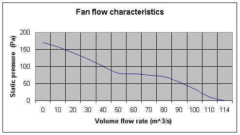
Figure 4.4 An example of the Fan flow characteristics
If your requirement is to choose the fan which will be appropriate for the equipment you are designing, you may need to perform 'system curve' simulation (see section 4.1.1) in order to obtain the 'system characteristics' which would then be used to determine the fan 'operating point' which occurs at the intersection of the system curve with the fan characteristic curve.
The 'Fan operating point' option in 'Models' menu in FLAIR automates this procedure; you are only required to specify the fan characteristic curve in tabulated form, and FLAIR will calculate the 'operation point'.
When the "Fan operating point" option is activated, FLAIR will compute the fan operating point for a given fan characteristic curve using an iterative method as follows:
This option works in the same manner for a single fan and for multiple fans each having different characteristic curve.
Fans in parallel are treated as separate fans with the combined characteristics of each fan. Fans in series are treated as a single fan with the combined characteristics.
At the end of the result file, you will find information about the operating point of your fan-system combination.
Note that fan-setting cannot be active at the same time as system-curve calculation; therefore when you activate fan-setting, if system-curve is active it will be automatically de-activated. At least one FAN object must exist before this option can be activated.
How FLAIR stores the fan flow characteristic curve
The fan flow characteristic curve is stored in a file called 'FANDATA'. The file can contain information for up to 50 fans. The format for each fan is:
Fan title (up to 16 characters).
Number of data pairs for the fan (single integer up to 100).
Two columns of numbers: first column is flow-rate in m^3/h; and second column is pressure-drop in Pa.
Example of Fan data
FAN1
5
0.   8.
30. 6.
60. 4.
90. 2.
120. 0.
It shall reside in the current working directory.
When 'Fan operating point' is active, a 'Settings' button appears, which leads to this page:
Figure 4.5 The Fan Operating Point Settings panel.
To use the "Fan Operating point" option, you need to do the following:
In section 6.6, there is a tutorial example which provides step-by-step instructions on how to activate the "Fan Operating Point" option for a single fan mounted at a boundary of a cabinet.
The 'Solve pollutants - Settings button leads to the following panel:
Figure 4.6 The Solve Pollutants Settings panel.
This panel allows up to five additional concentration equations to be solved. These can represent whatever the user wishes - often they will be concentrations of a pollutant species, perhaps CO released from vehicle exhausts. The names of these variables are at the user's choice, up to four characters. The default names are C1, C2, C3, C4 and C5.
When activated, each variable is set to:
All of these can be changed later. The nominal units of these equations are kg/kgmixture, but they can represent a wide range of quantities.
Note that the first pollutant is the C1 variable used in the Ideal Gas Law with mixture gas Constant available for the gas density from the 'Properties' panel. If the 'Include in gas density calculation' button is set to YES, the dialog changes to that shown in Figure 4.6a:
Figure 4.6a The Solve Pollutants Settings panel.
The molecular weight of each species, and that of the carrier fluid, can now be set. These will be used to calculate a mixture molecular weight which is then used in the Ideal Gas Law to obtain the fluid density. The mixture molecular weight is placed in the STOREd variable GMIX for plotting in the Viewer. The formula used to obtain the mixture molecular weight is:
GMIX = Mc(1-nCi)+nMi Ci
where Mc and Mi are the molecular weights of the carrier and species respectively.
The density is then calculated from:
r = (P1+PRESS0)*GMIX/(8314.46*(TEM1+TEMP0))
where PRESS0 is the 'Reference pressure' set on the Main Menu, Properties Panel, and TEMP0 is 273 if 'Temperature units' on that panel is set to 'Centigrade' or 0.0 if it is set to 'Kelvin'. P1 and TEM1 are the solved-for pressure and temperature.
The aerosol model assumes a very dilute particle phase (one-way coupling) with no collisions or coalescence, and drift-flux modelling is used to represent slippage between the particle and gas phases due to gravitational effects. In practice, aerosols can be deposited on surfaces by various mechanisms, including particle inertia, gravitational settling, Brownian diffusion (where particles are transported towards the surface as a result of their collisions with fluid molecules), turbulent diffusion (where particles are transported towards the surface by turbulent flow eddies), turbophoresis (where particles migrate down decreasing turbulence levels as a result of interactions between particle inertia and inhomogeneities in the turbulence field) and thermophoresis (where temperature gradients drive particles towards or away from surfaces).
The PHOENICS model27 considers all these mechanisms apart from thermophoresis. The surface-deposition fluxes themselves are calculated by using semi-empirical wall models as a function of particle size, density and friction velocity, and the deposition rates are reported automatically for all surfaces by the CFD solver in the RESULT file.
Typical applications include studying indoor air quality and designing ventilation systems to deal with: human exposure to biological or radiological aerosols in healthcare or laboratory environments; health hazards from industrial aerosols; protective environments and isolated clean rooms; and surface contamination of artworks, electronic equipment, etc.
The 'Solve aerosols - Settings button leads to the following panel:
Figure 4.6b The Solve Aerosols Settings panel.
This panel allows up to five additional aerosol concentration equations to be solved. These can represent whatever the user wishes. The names of these variables are at the user's choice, up to four characters. The default names are C6, C7, C8, C9 and C10.
When activated, each variable is set to:
All of these can be changed later. The nominal units of these equations are kg/kg mixture, but they can represent a wide range of quantities. It is often convenient to solve for aerosol concentration normalised by the inlet value. This entails setting the inlet value to 1.0.
The 'Store' buttons allow several derived quantities to be STOREd for each species:
These can then be displayed as contours and surface contours in the Viewer.
The deposition model (common to all species) is chosen as shown below:
Figure 4.6c Deposition Models
The two options with marked '(Y+ > 30)' assume that the near-wall cell is in the turbulent zone, and so may not produce reliable results in regions of low turbulence. The last option is independent of Y+ and so can be used in regions of low turbulence. However, it does not include turbophoresis.
If the 'Solve smoke mass fraction' button is switched to 'ON', FLAIR will solve an equation for the mass-fraction of a passive contaminant, usually the products of combustion from a fire.
If the 'Solve smoke mass fraction' button is set to ON, the parameters controlling the smoke production by the fire can be set from the 'settings' menu as shown in figure 4.7.
Figure 4.7 Smoke production parameters
Note that there three standards for the release of smoke. These are:
The 'International' method is a general smoke generation model, and can be used for many kinds of fires. The Dutch and Belgian standards are aimed at modelling car fires in car parking garages, and are not suitable for other applications.
4.6.1 'International' Fire Standard
The parameters are:
The default values were derived from experiments on the burning of a car vehicle using a Heat Release Rate (Qt) of 6MW, and a Heat of Combustion (Hfu) of 25 MJ/kg.
The total heat release rate Qt, mass consumption rate of fuel Mf and heat of combustion Hfu are linked by:
Qt = h * Mf * Hfu
where h is the combustion efficiency. The Heat of Combustion to be entered is an effective Heat of Combustion, in that it already includes h.
The mass generation rate of product is then derived from
Mp = (1+Rox) * Mf
For example, when the fire mass source is set to 'Heat related', the following expression is used:
Mp = Qt * (1+Rox) / Hfu
If the radiation model is not used, the heat release to the fluid domain should be reduced by the radiative fraction Rf (the portion of heat which is transferred directly by radiation). The CIBSE Guide E [20034] indicates that (1-Rf) is of the order 1/1.5 (=0.6667) i.e. Rf=0.33333.
The heat release set for the FIRE object is the total heat, Qt. This is used to deduce the smoke mass source, but is multiplied by(1-Rf) for use as the convective heat source. Strictly speaking, the radiative part of the heat release should be spread over the surrounding surfaces, but this is rarely done in practice.
If the radiation model is used, Rf is set to 0.0, as the partitioning between radiative and convective transfer is being modeled.
4.6.2 Dutch NEN6098 Fire Standard
4.6.2.1. Introduction
NEN6098 provides guidelines in the Netherlands for the design of smoke control systems for mechanically-ventilated car parks. Appendix B of NEN 6098:2012 covers the requirements for CFD analysis, and includes information for the specification of the heat-release and smoke-generation rates, and formulae for determination of the optical density and visibility distances.
4.6.2.2. Heat release rate
The standard specifies the total heat release rate as a function of time for a fire associated with 3 cars, as shown in Figure 2.1 and tabulated here.
The standard states that the second car will start burning 10 minutes after the ignition of the first car, and the third car will burn 5 minutes after the second car ignites. The fire curve of one burning car is based on measurements performed by TNO28, which can be seen in fire curves shown above reproduced from the standard.
The specified heat release rate includes both the convective and radiative contributions, and the standard specifies a radiative fraction Rf =0.3 (the portion of heat which is transferred directly by radiation). If a thermal-radiation model is not used in the CFD simulations, then the heat release rate to the fluid domain should be reduced by this amount.
4.6.2.3. Smoke production rate
The smoke production rate as products is computed from the following formula:
Mp = Qt * (1+Rox) / Hfu
If the radiation model is not used, the heat release to the fluid domain is automatically reduced as stated above.
4.6.3 Belgian NBN S 21-208-2/A1 Fire Standard
4.6.3.1. Introduction
The Belgian Standard NBN S 21-208-2/A1 gives guidelines for the CFD analysis of fires of cars in parking garages. It does not consider heat exchange between the hot smoke and the surrounding structures. In PHOENICS terms, all blockages should be of non-participating material 198.
4.6.3.2. Heat release rate
The heat release rate from 1 or 2 cars burning is specified in the standard. The curves are shown below:
They are tabulated here and here
The specified heat release rate includes both the convective and radiative contributions, and the standard specifies a radiative fraction Rf =0.34 (the portion of heat which is transferred directly by radiation). If a thermal-radiation model is not used in the CFD simulations, then the heat release rate to the fluid domain should be reduced by this amount.
4.6.3.3. Smoke production rate
The smoke production rate as products is computed from the following formula:
Mp = Qt / Hfu
If the radiation model is not used, the heat release to the fluid domain is automatically reduced as stated above.
The treatment of Optical Density and Sight length is much like the International treatment described below. A difference is the interpretation of the SMOK variable. In the Belgian standard it is taken to be the mass concentration of smoke particulates directly, so there is no reference to the stoichiometric ratio Rox. This is implemented by setting Rox to zero and not exposing it to the user.
4.6.4 Optical smoke density - International
The smoke resulting from a fire is associated with reduced visibility owing to the light scattering and absorption properties of the soot particles. Therefore, only a certain fraction of light can pass through the smoke, and the optical density of smoke provides a measure of the light obscuration properties of the solid particles. The fraction of light passing through a smoke layer of a given thickness L is given by the Beer-Lambert law [Tuomisaari, 199716], which can be expressed as:
I/Io = 10(-DL) (1)
where I is the intensity of light in the presence of smoke, Io is the intensity in the absence of smoke, L is the optical path length, and D is the optical density with units of m-1. The above equation can also be expressed in terms of natural logarithms [Tuomisaari, 199716], so that:
I/Io = e(-KmCs,pL) (2)
where Km is the mass specific extinction coefficient of the smoke aerosol in m2/kg, and Cs,p is the mass concentration of the smoke aerosol in kg/m3:
PHOENICS-FLAIR solves for the mass-fraction variable SMOK, which represents the mass fraction of smoke as products of combustion Cs in kg-smoke/kg. The mass concentration of particulate smoke Cs,p is computed from:
Cs,p = ρ Ys Cs /(1+Rox) (3)
where ρ is the mixture density, Ys is the particulate smoke yield in kg-smoke/kg-fuel, and Rox is the stoichiometric coefficient in kg-oxygen/kg-fuel. The value of Rox can be derived by assuming that
Hfu= b Rox (4)
where Hfu is the heat of combustion of the fuel (J/kg), and b is an empirical constant reported to be within �5% of 13.1MJ/kg-fuel for most common combustible species (Babrauskas et al [198513, 199211,12] ). From equations (1) to (3), it follows that the smoke optical density is given by:
D = Km Cs,p/2.3 = Kmρ Ys Cs /(2.3 (1+Rox)) (5)
In the literature, it has been established empirically that the value of Km can be considered as a constant the order of 7000 to 8000 m2/kg [4,7,8]. For example, these references suggest the value of 7600 m2/kg for the flaming combustion of both wood and plastics.
The optical density is made available for plotting in the Viewer as the variable OPTD.
4.6.5 Visibility - Sight length or Visibility distance - International
The visibility in smoke is defined as the furthest distance δ at which an object can be perceived, and it is computed from [4,5]:
δ = A / (KmCs,p) (6)
where A is an empirical coefficient with A=3 for light-reflecting signs, and A=8 for light-emitting signs [4,5]. Light emitting objects such as electric lights or illuminated signs are more easily perceived than light-reflecting objects which receive ambient illumination.
The relationship between visibility distance and optical smoke density can be deduced from equations (5) and (6) as:
δ = A / (2.3 D) (7)
The CIBSE fire-engineering guide [4] suggests that people are reluctant to proceed through smoke if the visibility is less than 8m, and so for the purposes of escape, the visibility should be at least this value.
In PHOENICS-FLAIR the sight length (or visibility) is calculated according to:
SLEN = min(Dmax, δ)
The visibility coefficient Dmax is defaulted to 30.0m, and this simply ensures that the sight-length has a finite rather than infinite value in smoke-free regions.
Two sight length variables are provided, SLEN which has A defaulted to 3.0, and SLN2 which has A defaulted to 8.0.
In earlier versions of FLAIR (pre 2008), the sight length was defined as:
SLEN = min(C, A'/(B*ρ*SMOK))
The default values employed by PHOENICS for the visibility coefficients A' and B were related to car fires in parking garages with sufficient supply of air. The smoke production & potential in an air-poor environment ( a car in a small garage or several cars burning together) will be significantly higher.
The coefficient B which took the value of 137 was computed from a smoke potential SP of 400m2/kg and a stoichiometric ratio Rox of 1.923 kg oxygen per kg of fuel (B=SP/(1+Rox)). The values of SP and Rox were derived from experiments on the burning of a car vehicle using a Heat Release Rate (Q) of 6MW, and a Heat of Combustion (H) of 25 MJ/kg. A' was 1 for light-reflecting objects and 2.5 for light-emitting objects.
Comparing the sight length formulae, we see that
Ys = A * B * (1+Rox)/(A' * Km)
Taking A=3; B=137, Rox=1.923, A'=1.0 and Km=7600, we get Ys=0.158
Further smoke-potential values can be found in the literature (see for example Drysdale [20009] and Hushed [200410]).
The visibility coefficient C is now Dmax.
4.6.6 Optical Density and Visibility Distances - Dutch NEN6098
The standard uses the smoke potential rather than the smoke yield as the basis for determining the optical density and visibility distances. For most solid burning materials, a smoke potential SP of 200-400 m2/kgfuel is reported in the literature29. The standard states a value of SP=400 m2/kgfuel should be used for the smoke potential, and that the visibility distances should be computed from:
δ = A / D
where A=1.0 for light-reflecting objects & A=2.5 for light-emitting objects. The optical density D in units of m-1 is given by:
where ρ is the gas mixture density, Cs is the mass fraction of smoke as products in kgsmoke/kg, and k is the extinction coefficient in m2/kgsmoke:D= kρCs
where Rox is the stoichometric ratio given as Rox=1.92 kgoxygen/kgfuel by NEN-6098..k = SP/(1 + Rox)
4.6.7 Light Intensity Reduction
An alternative to sight length is to calculate the reduction in light intensity due to the smoke. The Beer-Lambert Law can be used to deduce the effect of the smoke on light intensity
LR = 100.* Iz / Io
= 100.*e ( - S ( Cs*r*Km * dz) )
where dz is the distance along the path from a point to the point being looked at. Iz is the light intensity at the current point, and Io is the intensity at the origin. LR is then the percentage reduction in light intensity. When the light intensity is reduced to less than 0.16% of the original, the object is no longer visible.
In FLAIR, this has been implemented as a post-processing option in the Viewer. Starting at the probe, an integration is carried out along straight lines between the probe and each cell centre. A variant of the particle tracking routine is used for this purpose. Whenever a solid cell or blocked face is encountered, the integration is stopped and the intensity ratio is set to 0.0, as the probe cannot be seen from further along that path.
For a fine grid, the calculation can be quite lengthy as in principle the number of integrations is NX*NY*NZ-1. If some areas can be guaranteed not to be visible e.g. other floors, some time can be saved by restricting the plotting range to exclude the unwanted areas. To do this, go to the 'Plot Limits' tab of the Viewer Options dialog and set the volume for plotting (and integrating).
The steps in activating and displaying the light reduction ratio are:
Figure 4.8 The Viewer Domain Dialogue Box.
In the above image, the fire is not visible from anywhere to the right of the iso-surface, either because the view is blocked by the plate object, or because it is obscured by the smoke.
4.6.8 Derived quantities
In addition to the solved-for combustion-products mass fraction (SMOK), the two sight length variables SLEN and SLN2 and the optical density OPTD, the following derived quantities can be calculated and stored:
where Yco is the CO yield in kg-CO/kg-fuel.
4.6.9 Fire products data
For various fire materials, Table 4.6.9.1 provides suggested values of heats of combustion and yields of smoke particulates and carbon monoxide ( see CIBSE Guide E [20034] )
| Material | Hfu (MJ/kg) | Yco (kg/kg) | Ys (kg/kg) |
| Timber | 13.0 | 0.020 | <0.01 - 0.025 |
| PVC- Polyvinyl chloride | 5.7 | 0.063 | 0.12 - 0.17 |
| PU- Polyurethane (flexible) | 19.0 | 0.042 | <0.01 - 0.23 |
| PU- Polyurethane (rigid) | 17.9 | 0.18 | 0.09 - 0.11 |
| PS- Polystyrene | 27.0 | 0.060 | 0.15 - 0.17 |
| PP- Polypropylene | 38.6 | 0.050 | 0.016 - 0.1 |
Table 4.6.9.1 Fire data for flaming combustion
Heat release rates, heats of combustion and yields for other materials can be found in the literature. For example, Babrauskas et al [198513, 199211,12] examined the fire behaviour of upholstered furniture, and found that the data reported varied considerably with the component materials for the frame, cushioning material and upholstery fabric. Typical values for a traditional upholstered easy chair are Hfu=18MJ/kg, Yco=0.05kg/kg and Ys=0.025kg/kg. NFPA 92B [20056] lists heats of combustion and heat release rates for a large number of combustible materials.
The stoichiometric ratio Rox can be estimated from the heat release rate Q by assuming that the heat released per unit mass of oxygen is constant ( Huggett [198014] ). In the literature, this ratio Hfu/Rox is taken as 13.1 MJ/kg and varies by only �5% for almost any common combustibles ( Babrauskas et al [198513, 199211,12] )
If the 'Solve Specific humidity' button is switched to 'On'. the specific humidity equation, MH2O, will be solved. The variable, MH2O has units of kg water vapour/kg mixture. It is a mass fraction of water vapour.
By clicking on 'settings', the dialog box shown in figure 4.9 will appear.
Figure 4.9 Humidity settings dialog
Several derived quantities can be displayed. These are:
This has units of grams of water per kilogram of air.
If the Humidity ratio button is set to On, the humidity ratio in g/kg will be derived. The variable name for plotting in the Viewer is HRAT.
If the Relative humidity button is set to On, the relative humidity in % will be derived. In this case, the water-vapour saturation pressure, partial pressure and mole fraction are also made available for storage as shown in figure 4.10.
Figure 4.10 Relative humidity dialog box
The variable name for plotting in the Viewer is RELH.
As seen from figure 4.10, if the relative humidity is activated, the following quantities which are used in the derivation of relative humidity can also be stored:
The Wet Bulb temperature is the temperature of adiabatic saturation. This is the temperature indicated by a moistened thermometer bulb exposed to the air flow.
Wet Bulb temperature can be measured by using a thermometer with the bulb wrapped in wet muslin. The adiabatic evaporation of water from the thermometer and the cooling effect is indicated by a "wet bulb temperature" lower than the "dry bulb temperature" in the air. (The Dry Bulb Temperature refers basically to the ambient air temperature.)
The rate of evaporation from the wet bandage on the bulb, and the temperature difference between the dry bulb and wet bulb, depends on the humidity of the air. The evaporation is reduced when the air contains more water vapor.
The wet bulb temperature is always lower than the dry bulb temperature but will be identical with 100% relative humidity (the air is at the saturation line).
In FLAIR, the wet bulb temperature is derived from the dry bulb temperature and the relative humidity using the following equation taken from Stull [201119]:
Twet = Tair atan[0.151977(RH+8.313659)1/2 + atan(Tair+RH) - atan(RH-1.676331)+0.00391838(RH) 3/2 atan(0.023101RH) - 4.686035
where Tair is the dry bulb temperature TEM1 and RH is the relative humidity as a percentage, RELH. The equation is valid for a pressure of 101.325kPa and the combinations of dry-bulb temperatures and relative humidities shown in the image below:
The variable name for plotting in the Viewer is TWET. The maximum air temperature used in the derivation of Twet is 50 deg C.
The Dew Point is the temperature at which water vapor starts to condense out of the air (the temperature at which air becomes completely saturated). Above this temperature the moisture will stay in the air.
In FLAIR, the Dew Point-temperature is calculated from the Magnus Equation, with constants taken from Alduchov & Eskridge [1996 20]
Tdew = 243.04(ln(RH/100)+17.625Tair/(243.04+Tair))/(17.625-ln(RH/100)-17.625Tair/(243.04+Tair))
where RH is the relative humidity in % RELH, and Tair is the dry-bulb temperature TEM1.
The variable name for plotting in the Viewer is TDEW.
The units used to specify boundary sources (inlets, openings, volume sources at BLOCKAGE objects, area sources at PLATE objects) can be set on the dialogs for the individual objects.
The options are:
The default is Specific Humidity
FLAIR provides for several comfort index calculations:
Clicking on the Comfort Index button leads to a panel where any or all of the calculations can be activated, and relevant input parameters set.
Figure 4.11 The Comfort index dialog box
This is just the air temperature in the air space. The standard temperature display in the Viewer includes the temperatures of any participating solids, so it can be difficult to determine the air temperature precisely. TAIR is not evaluated or plotted inside any solid.
Thermal comfort index, or dry resultant temperature, is a standard index used to show the level of comfort within the occupied space. It is a function of air temperature, air velocity and mean radiant temperature. The formula as defined in Volume A of the CIBSE Guide is:
Tres = ( Trad + Tair * (10*vel) 0.5) /( 1+ (10* vel) 0.5)
Where Tres is the resultant temperature; Trad mean radiant temperature; Tair air temperature; vel air velocity.
The mean radiant temperature can be a user-set constant value, or can be taken to be the T3 radiation temperature of the IMMERSOL radiation model.
Comfortable values of Tres are typically in the range 16-28 deg C, depending on the external conditions and type of occupancy.
Apparent Temperature is a general term for the perceived outdoor temperature, caused by the combined effects of air temperature, relative humidity, radiation and wind speed.
The formulae for the Apparent Temperature used in PHOENICS-Flair are those used by the Australian Bureau of Meteorology. They are an approximation of the value provided by a mathematical model of heat balance in the human body. They can include the effects of temperature, humidity, wind-speed and radiation.
Two forms are given by the Australian Bureau, one including radiation and one without.
The expression without radiation is suitable for the working condition of people walking in the shade; the expression with radiation is suitable for the working condition of people in direct sunlight.
The TAPP Apparent Temperature is the non-radiation version. The expression used is:
AT = Ta + 0.33�e - 0.70�ws - 4.00
where:
Ta = Dry bulb temperature (C) (TEM1 in PHOENICS-Flair)
e = Water vapour pressure (hPa) [humidity]
ws = Wind speed (m/s) at an elevation of 10 meters (taken to be the local VABS in PHOENICS-Flair)
The vapour pressure e is calculated from the temperature and relative humidity using the equation:
e = rh / 100 � 6.105 � exp ( 17.27 � Ta / ( 237.7 + Ta ) )
where:
rh = Relative Humidity [%] (RELH in PHOENICS).
The variable name used to store the non-radiative AT is TAPP.
The TAPR Apparent Temperature includes the radiation term. The expression used is:
AT = Ta + 0.348�e - 0.70�ws + 0.70�Q/(ws+10.0) - 4.25
where:
Q = Net radiation absorbed per unit area of body surface (w/m2)
and the other terms are as defined above.
Steadman, 197321 indicates that Q is likely to be in the range -20 to 130 W/m2.
The variable name used to store the AT is TAPP.
Note that in order to calculate either Apparent Temperature, the solution of Specific Humidity and the derivation of Relative Humidity must both be turned on.
The Universal Thermal Climate Index UTCI provides an assessment of the outdoor thermal environment in bio-meteorological applications based on the equivalence of the dynamic physiological response predicted by a model of human thermoregulation, which is coupled with a state-of-the-art clothing model. The operational procedure, which is available as software from the UTCI website (www.utci.org), shows plausible responses to the influence of humidity and heat radiation in the heat, as well as to wind speed in the cold and is in good agreement with the assessment of ergonomics standards concerned with the thermal environment.
The necessary research for this was conducted within the framework of a special commission of the International Society of Biometeorology (ISB) and European COST Action 730.
The published subroutine returns the UTCI as a function of air temperature, water vapour pressure, mean radiant temperature and wind speed 10m above ground level. In the Flair implementation, the local air temperature is taken to be the solved temperature TEM1, the local water vapour pressure is derived from the solved water vapour mass fraction MH2O or from a user-set constant, the local mean radiant temperature is taken as the solved radiant temperature T3 or a user-set constant, and the wind speed is taken to be the local absolute velocity VABS.
The PET comfort index, derived from the human heat balance model, combines weather and thermo-physiological parameters (clothing and human activities). It is used to measure the thermal comfort of an individual in a given situation by comparing their physiological responses to those they would have in the reference environment, for example an office in which they feel generally comfortable.
For the study of indoor spaces, the PET index is often used as its reference environment is comparable to an office and it is easier to apply and less theoretical than the Universal Thermal Climate Index (UTCI).
The published subroutine (https://palm.muk.uni-hannover.de/trac/browser/palm/trunk/SOURCE/biometeorology_pet_mod.f90?rev=3467&order=author) returns the PET index as a function of air temperature and pressure, water vapour pressure, mean radiant temperature and wind speed 1.1m above ground level. In the Flair implementation, the local air temperature is taken to be the solved temperature TEM1, the local water vapour pressure is derived from the solved water vapour mass fraction MH2O or from a user-set constant, the local mean radiant temperature is taken as the solved radiant temperature T3 or a user-set constant, and the wind speed is taken to be the local absolute velocity VABS.
Other assumed inputs are for a standing male aged 35, height 1.75m, weight 80kg, metabolic rate 80W (1.4mets, sedentary, or light standing activity) and clothing insulation 0.9clo.
The Thermal Sensation Index (TSI) is an empirical model developed by studies conducted in the context of Japan. It considers five climatic factors� air temperature, horizontal solar radiation, wind speed, relative humidity and mean radiant temperature� at a given location and time. TSI�s prevalence in Hong Kong can be explained by its user-friendly nature. Particularly, it is the index that public housing projects in Hong Kong adopt.
TSI is subdivided into a scale of seven levels, where level 1 is cold, and level 7 is hot. While level 4 is considered neutral, a TSI between 3 and 5 is deemed thermally acceptable, where no major discomfort is expected.
TSI can be calculated by the following formula:
TSI = 1.7 + 0.1118Ta + 0.0019SR � 0.322WS � 0.0073RH + 0.0054ST
Where,
Ta = air temperature (�C)
SR = horizontal solar radiation (W/m2)
WS = wind speed (m/s)
RH = relatively humidity (%)
ST = surrounding ground surface temperature (�C), assumed to be Ta+3�C for TSI calculation
We have implemented a simplified version according to BEAM Plus New Buildings Version 2.030. In the simplified BEAM implementation, the following values are assumed constant:
Ta = air temperature (�C) = 31�C
SR = horizontal solar radiation (W/m2) = 254W/m2 in shadow, 525W/m2 in the sun
WS = wind speed (m/s) = VABS as calculated by PHOENICS-Flair
RH = relatively humidity (%) = 72%
ST = surrounding ground surface temperature (�C), assumed to be Ta+3�C for TSI calculation
PMV is an index defined in ISO 7730 that predicts the mean value of the votes of a large group of people on a 7-point thermal sensation scale:
+ 3 hot
+2 warm
+1 slightly warm
0 neutral
-1 slightly cool
-2 cool
-3 cold
Figure 4.12 PMV settings box
For the PMV option, the following input parameters are required:
The radiant temperature - this can be a user-set constant value, or can be taken to be the T3 radiation temperature of the IMMERSOL radiation model.
The clothing insulation - clothing insulation is measured in
'clo' (clothing unit)
'tog' (European unit of thermal insulation) or
m2 k/w
where
1 clo = 0.155 m2 k/w
1 tog = 0.645 clo
The practical range is between 0 clo (no clothing) and 4 clo (Eskimo clothing); 1lb (0.454kg) corresponds roughly to 0.15 clo, with 0.6 clo and 1.0 clo being typical of summer and winter clothing respectively.
The default value is 0.6 clo.
The Metabolic Rate - is measured in 'met' (metabolic units) or W/m2; 1 met = 58.15 W/m2. The appropriate value depends on the activity being undertaken (see ISO 7730 and ISO 8996):
0.8 met - reclining
1.0 met - seated, relaxed
1.2 met - sedentary activity (office, dwelling, school, laboratory)
1.6 met - standing, light activity (shopping, laboratory, light industry)
2.0 met - standing, medium activity (shop assistant, domestic work, machine work)
1.9 met - walking on the level at 2 km/h
2.4 met - walking on the level at 3 km/h
2.8 met - walking on the level at 4 km/h
3.4 met - walking on the level at 5 km/h
The default value is 1.2 met.
The external work - is the part of the metabolic rate that is used up in the activity being performed, rather than contributing to the heat balance of the individual concerned. It is usually taken as zero, and should always be less than the metabolic rate.
The default value is 0.0.
The relative humidity - individual comfort is influenced by the humidity of the air, which affect the heat loss through the skin. It is often sufficient to specify a reasonable value for a particular environment, but it is also possible to calculate the humidity as part of the simulation.
If humidity is calculated it is important to specify realistic conditions at domain inlets and at sources (people, surfaces).
The default value is 50%.
PPD is an index defined in ISO 7730 that predicts the percentage of a large group of people who are likely to feel too warm or too cool, i.e the percentage of a large group of people who would vote for values other than 0, -1 or +1 on the thermal sensation scale used for PMV.
The required input parameters are the same as for PMV.
PPDR is defined in ISO 7730 as the percentage of people dissatisfied due to draught, using the following equation:
PPDR = (34-Ta)*(V-0.05)0.62*(0.37*V*I+3.14)
where Ta is the local air temperature, V is the local air velocity and I is the local turbulence intensity in %. In FLAIR, it is derived from the local turbulence quantities and the local absolute velocity.
I = 100*k0.5/V
where k is the local turbulent kinetic energy (KE).
PLOS, the loss in performance in % by people occupying the space, is defined by Roelofsen3 as:
PLOS = b0 + b1PMV + b2PMV2 + b3PMV3 + b4PMV4 +b5PMV5 + b6PMV6
where PMV is the local Predicted Mean Vote and the regression coefficients b1 - b6 are given in the table below:
| Regression coefficient |
Cold side of comfort zone |
Warm side of comfort zone |
| b0 | 1.2802070 | -0.15397397 |
| b1 | 15.995451 | 3.8820297 |
| b2 | 31.507402 | 25.176447 |
| b3 | 11.754937 | -26.641366 |
| b4 | 1.4737526 | 13.110120 |
| b5 | 0.0 | -3.1296854 |
| b6 | 0.0 | 0.29260920 |
The wet bulb globe temperature (WBGT) index is the most widely used and accepted index for the assessment of heat stress in industry. It has been published as British Standard BS EN 27243.
The WBGT index is an empirical index. It represents the heat stress to which an individual is exposed. The index was developed specifically for use in industrial settings. The practicalities of an industrial application necessitated a compromise between the requirement for a precise index and the need to be able to easily take controlled measurements. The WBGT should be used to estimate whether or not a problem exists, by identifying if the reference values are exceeded by the measured values. When the reference values are exceeded, a more advanced index (BS EN 12515 - Required Sweat Rate) should be used to provide a more accurate estimation of heat stress.
The WBGT-index combines three measurements:
The following illustrates the relationship between the different measurements.
Inside buildings and outside buildings without experiencing the effects of radiation from the sun (solar load):
WBGT = 0.7tnw + 0.3Ta
Outside buildings with solar load, or where a radiant heat source is present indoors:
WBGT = 0.7tnw +0.2tg +0.1ta
where tnw is TWET, Ta is TEM1 and tg is the Immersol radiation temperature, T3.
When set to 'ON', a 3D variable named CP is created, and the solver fills it with values of the local pressure P1, divided by the dynamic head at the wind reference height. This is obtained from the attributes of a WIND object. If there is no WIND object, the CP store will not be filled.
When set to 'ON', a 3D variable named TINS is created. The solver fill it with values of the local turbulence intensity defined as:
Tins = 100 * k0.5/Vabs
If the LVEL model is being used, k is evaluated from
k = νt/(Cμ*l)where l is the turbulent length scale.
The "Mean age of air" measures the time in seconds that the air has taken to travel from entry to the domain to reach the point in question. It is represented by the variable AGE.
First consider a couple of basic cases.
The principal use of mean age of air is to highlight regions of the domain which are poorly ventilated. If there are stagnant areas or regions with recirculation, the mean age of air in these areas is likely to be large - quite possibly larger than the age at outflow. The age of air increases as it recirculates; this increase is limited by turbulent diffusion, which transports the high AGE values out of the recirculation.
Plotting AGE in the Viewer serves as a means of rapidly identifying poorly ventilated regions. As an example, consider a case where air enters a room through an aperture in one of the walls, and exits through another in the ceiling. The AGE in the farther half of the room, and the age at exit, are about 500s. But the red band along the left wall shows that the ventilation there is relatively poor, with an AGE of about 1000s.
Thus far we have considered the qualitative aspects of the age-of-air distribution. But in some cases the quantitative values may be of interest. This is often in safety-critical situations. For example, in an incinerator flue, it may be necessary for the flue gases to spend a specified minimum time within the flue, above a specified minimum temperature. Or to take another example, in a drinking-water reservoir, there may be a safety limit to the time that water can be retained in the reservoir; regions of high AGE (meaning age of water in this case) may represent a hazard.
In situations of this sort, some words of caution are required.
Pedestrian Wind Comfort Settings
When set to ON, as shown above, the measured wind statistics data in the 'Wind data file' will be used to show contour plots of the probability of encountering a wind speed higher than the one indicated by 'Threshold velocity' for the current wind direction. These probabilities can be shown in three forms:
The variable names for plotting in the VR-Viewer are NEN, PRO and PDAN. The probability of exceeding the threshold wind speed of 5 m/s is stored in PRO, and that of exceeding 15 m/s in PDAN.
| Activity | Band | Probability | Threshold Wind Speed |
| Roads and Car Parks | (A -> 1) | 6% | 10.95 m/s |
| Business walking | (B -> 2) | 2% | 10.95 m/s |
| Pedestrian walk-through | (C -> 3) | 4% | 8.25 m/s |
| Pedestrian standing | (D -> 4) | 6% | 5.6 m/s |
| Sitting | (E -> 5) | 1% | 5.6 m/s |
As the values of threshold wind speed and exceedance probability appear to differ in various publications, the above set of default values has been provided, with the option to change them.
Up to 6 threshold velocity / probability bands can be specified. The variable names for the individual probabilities of exceedance are PRO1, PRO2,...,PRONcrit, and LAWS for the criterion itself.
The 'Get Generalised Wind Climate File' button opens the Global Wind Atlas website. From here, wind data for large parts of the world can be downloaded in the form of Generalised Wind Climate Files.
Once the required area has been selected, download the GWC file from the 'Customised Areas' tab on the right of the screen. The file will appear in the Downloads area, with a .lib extension.
From the 'Wind data file' button browse to the downloaded file and select it. It may be convenient to copy or move the GWC file to the current working directory before opening it.
If the data format is selected as WEIBULL, and the data file specified has the file extension '.lib', then it will be treated as a GWC file. If the extension is anything else, it will be assumed that the file contains the exact coefficients already.
If a GWC file is detected, additional buttons appear:
to allow the specification of the Roughness class (Possible Values are: 0.00, 0.03, 0.10, 0.40, 1.50 m), and Height above ground (Possible values are: 10, 50, 100, 150 and 200 m) available in all GWC files.
The inlet wind speed used to generate the inlet profile is automatically taken to be the average velocity for the chosen sector:
Vsect = sum(Vi.prob)
where
Vi - the central velocity of the i'th speed bin
prob - probability of that bin
The reference height used for the inlet profile is taken to be the measurement height set in the wind speed data file.
The absolute velocity divided by the wind profile speed at the measurement height is then multiplied by the probability of wind in that sector and by the average measured velocity. This is STOREd in the variable VAV.
VAV = WRF * Vsect * sectP
where:
WRF = VABS/(wind profile speed at measurement height)
sectP = probability of wind in this sector
Vsect = sum(Vi*prob);
Vi = central velocity of i'th wind speed bin
prob = probability of that bin
After the last run has been made, the output files of all the runs must be passed through the PHISUM program which adds them all up. The VAV in the output file from PHISUM is then the average velocity over all sectors. When VAV is STOREd, the probability of exceeding the threshold (PRO) is also multiplied by sectP, so the PRO value in the summed file is the probability for all directions.
If the Dutch comfort index NEN8100 is used, the NEN values in the final summed file are recalculated based on the summed probabilities PRO and PDAN.
If the Lawson Criteria are used, the probabilities for each band will have been stored as PRO1,PRO2 etc. The LAWS values in the final summed file are recalculated from the summed PROn's, using threshold values read from Q1.
The PHISUM utility can be run from Run - Utilities.
See Section 5.8.3 of TR316 FLAIR-EFS User Guide for more details on the velocity averaging procedure.
FLAIR provides the IMMERSOL radiation model. When the Smoke model is on, it is likely that the absorptivity of the gas will be a function of temperature and/or smoke concentration. Options for this are provided on the Radiation Settings panel, shown in Figure 4.13.
Figure 4.13 Flair Radiation Settings panel
There are three options for setting the gas absorption:
Figure 4.14 Gas absorption settings
EMIS = const * SMOK
where const is a constant - by default 5.0 - and SMOK is the local smode concentration in kg/kg mixture.
EMIS = 0.01, if T < 323K and SMOK > 0.0001
EMIS = 0.01 + (3.49/377)(T- 323), if 323K <= T < 700K and SMOK > 0.0001
EMIS = 3.5 + (3.5/700)(T- 700), if T > 700K and SMOK > 0.0001
where T is the temperature in Kelvin. The test on SMOK > 0.0001 ensures that smoke-free zones behave as a transparent medium.
1. CIBSE Guide, Volume A, Design Data
2. ISO 7730 Second Edition 1994-12-15
Moderate thermal environments - Determination of the PMV and PPD indices and specification
of the conditions for thermal comfort.
3. Roelofsen, Paul. Journal of Facilities Management Volume 1, Number 3
November 2002 ISSN 1472-5967
The impact of office environments on employee performance: The design of the workplace as
a strategy for productivity enhancement
4. Fire Engineering CIBSE Guide E, ISBN 1 903287 31 6, CIBSE, London, (2003).
5. T.Jin, 'Visibility through fire and smoke', J.Fire & Flammability, Vol.9, pp135-155, (1978).
6. NFPA 92B, 'Standard for smoke management systems in malls, atria and large spaces', NFPA, Quincy, Massachusetts 02269-9101, USA, (2005).
7. G.W.Mulholland & C.Croarkin, 'Specific extinction coefficient of flame generated smoke', Fire & Materials, Vol.24, No.5, p227, (2000).
8. G.W.Mulholland, 'Smoke production and properties', Chapter 2, Section 13, p2-258, SFPE Handbook of Fire Protection Engineering, 3rd Edition, NFPA, Quincy, Massachusetts 02269-9101, (2002).
9. D.Drysdale, "An Introduction to Fire Dynamics", John Wiley, (2000);
10. B.P.Hushed, "Optical source units and smoke potential of different products" DIFT report 2004:1, DIFT, Denmark, (2004).
11. Babrauskas, V. "Generation of CO in Bench-Scale Fire Tests and the Prediction for Real-Scale Fires", Fire & Materials Int. Conf., Arlington, VA, USA, p155, (1992).
12. Babrauskas, V., J.R.Lawson, W.D.Walton & W.H.Twilley, "Upholstered furniture heat release rates measured with a furniture calorimeter", NBSIR 82-2604, USA (1992).
13. Babrauskas, V. & Krasny, J., "Fire Behaviour of Upholstered Furniture", NBS Monograph 173, NBS, USA(1985).
14. C.Huggett, 'Estimation of rate of heat release by means of oxygen consumption measurements', Fire & Materials, 4, 61-5, (1980).
15. Srebric, J., Chen Q., "Simplified Diffuser Boundary Conditions for Numerical Room Airflow Analysis", ASHRAE RP-1009, March 20, 2001
16. M.Tuomisaari, "Visibility of exit signs and low-location lighting in smoky conditions", VTT Publications 300, TRC of Finland, Espoo, (1997).
17. G.Heskestad & R.G. Bill, "Quantification of Thermal Responsiveness of Automatic Sprinklers Including Conduction Effects", Fire Safety Journal, 14:113-125, 1988.
18. A J Grandison, E R Galea, M K Patel. Fire Modelling Standards/Benchmark. Report on SMARTFIRE Phase 2 Simulations. Fire Safety Engineering Group, University of Greenwich, London SE10 9LS
19. Stull, R. 2011 Wet-Bulb Temperature from Relative Humidity and Air Temperature, American Meteorological Society November 2011.
20. Alduchov, O. A., and R. E. Eskridge, 1996: Improved Magnus form approximation of saturation vapor pressure. J. Appl. Meteor.,35,601-609.
21. Steadman, R. G. 1973: The Assessment of Sultriness. Part II: Effects of Wind, Extra Radiation and Barometric Pressure on Apparent Temperature. Journal of Applied Meteorology, Vol 18, p874-885
22. GENTRA User guide, CHAM TR/211.
23. Blocken, B., Briggen, P.M., Schellen, H.L & Carmeliet, J., "Intercomparison of wind-driven rain models based on a case study with full-scale measurements", 5th Int.Symp. on Computational Wind Engineering, Chapel Hill, North Carolina, USA May 23-27, (2010).
24. Foote G B and Du Toit P S: "Terminal Velocity of Raindrops Aloft". Journal of Applied Meteorology, 8, 249-253.
25. NEN 2006. Wind comfort and wind danger in the built environment, NEN 8100 (in Dutch) Dutch Standard.
26.Lawson TV. 1978. The wind content of the built environment. J Ind Aerodyn 3:93-105.
27 B.Zhao, C.Chen & Z.Tan, "Modelling of ultrafine partcle dispersion in indoor environments with an improved drift flux model", J. Aerosol Science, 40(1), p29-43, (2009).
28 N.J. Oerle, A.D. Lemaire, P.H.E. van de Leur, (1999) "Efficiency of thrust ventilation in closed car parks, Fire tests and simulations". TNO Report 1999-CVB-RR1442, (1999).
29 M.G.M. van der Heijden, "Heat and smoke removal in semi-open car parks", MSc Thesis, Eindhoven University of techmology, Eindhoven, Netherlands, (2010).
30 https://www.hkgbc.org.hk/eng/beam-plus/beam-plus-references/manuals-assessment/ManualsFiles/BEAMPlus_New_Buildings_v2_0(2021Edition).pdf
In addition to the simple example described in chapter 2, this chapter provides further 9 examples, each of which gives step-by-step instructions, combined with pictures, show how to use various features in FLAIR to set up models, to run the solver and to view the result. These cases are:
Tutorial 1 Investigating library case I203 illustrates how to load a case from the FLAIR library, to investigate the model settings, to run the case and to view the results.
Tutorial 2 A room with two radiators shows how to activate the IMMERSOL radiation model. The 'Duplicate object' function is used for the creation of the second window and radiator. The material of the radiators is selected from the property data base. A fixed heat flux is used as the heat source for the radiators.
Tutorial 3 Comfort indices in a room is similar to tutorial 2, but adds a chair and a sitting person into the room. This tutorial demonstrates how to activate the comfort index option.
Tutorial 4 Fire in a room shows how to use the Fire object for simulating a fire in a room. Smoke movement is also simulated.
Tutorial 5 A room with sunlight describes how to use Shapemaker to create a sunlight object in the model building.
Tutorial 6 A cabinet with a fan illustrates how to use the 'fan working point' option and how to create a fan-data file for the simulation.
Tutorial 7 Flow in a computer room shows how to use 'Group' and 'Arraying objects' features to add the desks and computers. The case also shows how to load a round diffuser from the predefined HVAC object library.
Tutorial 8 Flow over Big Ben demonstrates how to import a CAD file in STL format into the FLAIR VR-Editor to create the geometry. This tutorial also shows how to use a Wind_profile object to describe the wind profile at the upstream boundary. The 'Paint' object capability in the VR-Viewer is used to draw the pressure contours on the object surface.
Tutorial 9 Fire-spray in a compartment shows how to use the spray-head object and GENTRA module for the simulation of a fire-spray in a compartment. This kind of application of the sprinkler is commonly adopted in a car park for fire extinction.
Tutorial 10 Fire modeling gives an example of the FIRE object for a typical t2 fire in a simple configuration. It also shows how the operation of jetfans can be controlled by a temperature sensor using InForm.
Tutorial 11 Fire modelling - Car fire in a tunnel gives an example of the FIRE object for a typical car fire in a simple tunnel configuration.